, 82 min read
A Parsec-Scale Galactic 3D Dust Map out to 1.25 kpc from the Sun
Author
- Gordian Edenhofer (1,2,3)
- Catherine Zucker (3,4)
- Philipp Frank (1)
- Andrew K. Saydjari (3)
- Joshua S. Speagle (5,6,7,8)
- Douglas Finkbeiner (3)
- Torsten Enßlin (1,2) }
Institute
- Max Planck Institute for Astrophysics, Karl-Schwarzschild-Straße 1, 85748 Garching bei München, Germany
- Ludwig Maximilian University of Munich, Geschwister-Scholl-Platz 1, 80539 München, Germany
- Center for Astrophysics $\vert$ Harvard & Smithsonian, 60 Garden St., Cambridge, MA 02138
- Space Telescope Science Institute, 3700 San Martin Dr, Baltimore, MD 21218
- Department of Statistical Sciences, University of Toronto, Toronto, ON M5G 1Z5, Canada
- David A. Dunlap Department of Astronomy & Astrophysics, University of Toronto, Toronto, ON M5S 3H4, Canada
- Dunlap Institute for Astronomy & Astrophysics, University of Toronto, Toronto, ON M5S 3H4, Canada
- Data Sciences Institute, University of Toronto, Toronto, ON M5G 1Z5, Canada }
Abstract
Context. High-resolution 3D maps of interstellar dust are critical for probing the underlying physics shaping the structure of the interstellar medium, and for foreground correction of astrophysical observations affected by dust. }
Aims. We aim to construct a new 3D map of the spatial distribution of interstellar dust extinction out to a distance of 1.25kpc from the Sun. }
Methods. We leverage distance and extinction estimates to 54 million nearby stars derived from the Gaia BP/RP spectra. Using the stellar distance and extinction information, we infer the spatial distribution of dust extinction. We model the logarithmic dust extinction with a Gaussian Process in a spherical coordinate system via Iterative Charted Refinement and a correlation kernel inferred in previous work. We probe our 661 million dimensional posterior distribution using the variational inference method MGVI. }
Results. Our 3D dust map achieves an angular resolution of ${14'}$ ($N_\text{side}=256$). We sample the dust extinction in $516$ distance bins spanning 69 pc to 1250 pc. We obtain a maximum distance resolution of 0.4pc at 69pc and a minimum distance resolution of 7pc at 1.25kpc. }
Conclusions.
Our map resolves the internal structure of hundreds of molecular clouds in the solar neighborhood and will be broadly useful for studies of star formation, Galactic structure, and young stellar populations.
It is available for download in a variety of coordinate systems at https://doi.org/10.5281/zenodo.8187943 and can also be queried via the publicly available dustmaps Python package.
}
Key words. interstellar dust -- interstellar medium -- Milky Way -- Gaia -- Gaussian processes -- Bayesian inference }
- 1. Introduction
- 2. Stellar Distance and Extinction Data
- 3. Priors
- 4. Likelihood
- 5. Posterior Inference
- 6. Caveats
- 7. Results
- 8. Conclusions
- 9. ZGR23 in dust-free Regions
- 10. Metric Gaussian Variational Inference
- 11. Extinction Catalog
- 12. 2kpc Reconstruction
- 13. Using the Reconstruction
- 14. Literature
1. Introduction
Interstellar dust comprises only 1% of the interstellar medium by mass, but absorbs and re-radiates $>30%$ of starlight at infrared wavelengths (Popescu2002). As such, dust plays an outsized role in the evolution of galaxies, catalyzing the formation of molecular hydrogen, shielding complex molecules from the UV radiation field, coupling the magnetic field to interstellar gas, and regulating the overall heating and cooling of the interstellar medium (Draine2011).
Dust's ability to scatter and absorb starlight is precisely the reason why we can probe it in three spatial dimensions. It preferentially absorbs shorter wavelengths of a stellar spectrum, thus leading to stars behind dense dust clouds appearing reddened relative to their intrinsic colors. The amount by which stars behind dust clouds appear reddened allows us to infer the amount of dust extinction between us and the reddened star. In combination with distance measurements to reddened stars, we can de-project the integrated extinction measurements into a three-dimensional map of differential dust extinction.
Gaia has been transformative for the field by providing accurate distance information to more than one billion stars, primarily within a few kiloparsecs from the Sun. Precise distances not only improve our knowledge about a star's position, but they also break degeneracies inherent in the modeling of extinction and significantly reduce the extinction uncertainties (Zucker2019). Thanks to the large quantity of extinction and distance measurements available in the era of large photometric, astrometric, and spectroscopic surveys, we can now probe the 3D distribution of dust in the Milky Way on parsec scales.
A number of 3D dust maps combining Gaia and vast photometric and spectroscopic surveys already exist. These maps primarily differ in the way they account for the so-called fingers-of-god effect, or the tendency of dust structures to be smeared out along the line of sight (LOS). The effect stems from superior constraints on stars' plane-of-sky (POS) positions relative to their LOS distance uncertainties.
3D dust maps predominantly fall into two categories, each representing a trade-off between angular resolution and distance resolution: reconstructions on a Cartesian grid and reconstructions on a spherical grid. Cartesian reconstructions commonly feature less pronounced fingers-of-god but are lower in angular resolution (Vergely2022, Lallement2022, Lallement2019, Lallement2018, Capitanio2017) or encompass limited volumes of the Galaxy (Leike2020, Leike2019). Spherical reconstructions are often higher angular resolution and probe larger volumes of the Galaxy but come with more strongly pronounced fingers-of-god or similar artifacts (Green2019, Green2017, Rezaei2022, Rezaei2020, Rezaei2018, Rezaei2017, Chen2019, Chen2018, Dharmawardena2022, Leike2022).
Physical smoothness priors counterbalance the fingers-of-god effect as finger-like structures are a priori unlikely. In a Cartesian coordinate system it is comparatively easy to incorporate physical priors into the model such as the distribution of dust being spatially smooth. Smoothness priors are often incorporated using Gaussian Process (GP) priors. Sparsities and symmetries in the prior can be exploited to efficiently apply a GP on a regular Cartesian coordinate system.
Spherical coordinate systems break these sparsities and symmetries in the prior but are much better aligned with the desired spacing of voxels along the LOS. Nearby, voxels can be spaced densely while at greater distances voxels can be spaced further apart. Naively using a GP prior is infeasible and approximations either trade fingers-of-god artifacts for other artifacts (Leike2022) or are too weak to regularize the reconstructions (Green2019).
In this work, we present a 3D dust map that achieves high distance and angular resolution and probes a large volume of the Galaxy, all at a feasible computational cost. The map uses a new GP prior methodology to incorporate smoothness in a spherical coordinate system, mitigating fingers-of-god artifacts. With a spherical coordinate system we are able to probe dust beyond 1kpc while still resolving nearby dust clouds at parsec-scale resolution. In \Cref{sec:data}, we present the stellar distance and extinction estimates upon which our map is based. In \Cref{sec:priors}, we present our GP prior methodology for incorporating smoothness in a spherical coordinate system. \Cref{sec:likelihood} describes how we combine the data with our prior model and how we incorporate the distance uncertainties of stars. In \Cref{sec:posterior_inference} we describe our inference before recapitulating all approximations of the model and their implications in \Cref{sec:caveats}. Finally, in \Cref{sec:results} we present the final map and compare it to existing 3D dust maps and 2D observations.
2. Stellar Distance and Extinction Data
To construct a 3D dust map, we use the stellar distance and extinction estimates from Zhang2023, which are primarily based on the Gaia BP/RP spectra (spectral resolution R $\sim 30-100$). Zhang2023 adopt a data-driven approach to forward model the extinction, distance, and intrinsic parameters of each star given the combination of the Gaia BP/RP spectra and infrared photometry from 2MASS and unWISE (Carasco2021, DeAngeli2022, GaiaCollaboration2022, Montegriffo2022, Schlafly2019, Wright2010, Skrutskie2006). The model is trained using a subset of stars with higher resolution spectra ($R \sim 1800$) available with LAMOST (Wang2022, Xiang2022). The resulting catalog contains distance, extinction, and stellar type ($T_{eff}$, [Fe/H], $\log g$) information for 220 million stars. Throughout this work, we will denote the Zhang2023 catalog as ZGR23.
Compared to other stellar distance and extinction catalogs, the ZGR23 catalog features smaller uncertainties on the extinction estimates while still targeting a significant number of stars. Approximately 87 million ZGR23 stars have an $A_V$ uncertainty below $60$ mmag. Thus, ZGR23 achieves similar extinction uncertainties compared to the subset of $39,538$ stars in the StarHorse catalog (Queiroz2023) that have both higher resolution APOGEE spectra and Pan-STARRS1 (PS1; chambers2019) $grizy$ photometry (typical $A_V$ extinction uncertainty of $60$ mmag). While the ZGR23 catalog is limited to stars with Gaia BP/RP measurements, the quality of the data makes the inference from the ZGR23 catalog competitive with models based on catalogs with larger numbers of stars --- 799 million stars in Bayestar19 (Green2019), 265 million in StarHorse DR2 (Anders2019), and 362 million in StarHorse EDR3 (Anders2022). We further find the ZGR23 catalog to have fewer systematic shifts in the extinction and reliable extinction uncertainties based on an analysis in dust-free regions; see \Cref{appx:zgr23_in_dust_free_regions} for further details.
For our reconstruction we restrict our analysis to ZGR23 stars that have quality_flags<8 as recommended by the authors.
We further subselect the stars based on their distance.
We require ${1}/{(\omega-\sigma_\omega)}<1.8\,\hbox{kpc}$ and ${1}/{(\omega+\sigma_\omega)}>40\,\hbox{pc}$ with $\omega$ the parallax of a star and $\sigma_\omega$ the parallax uncertainty to enforce that all stars are likely within our reconstructed volume.
In total, we select 53,880,655 stars.
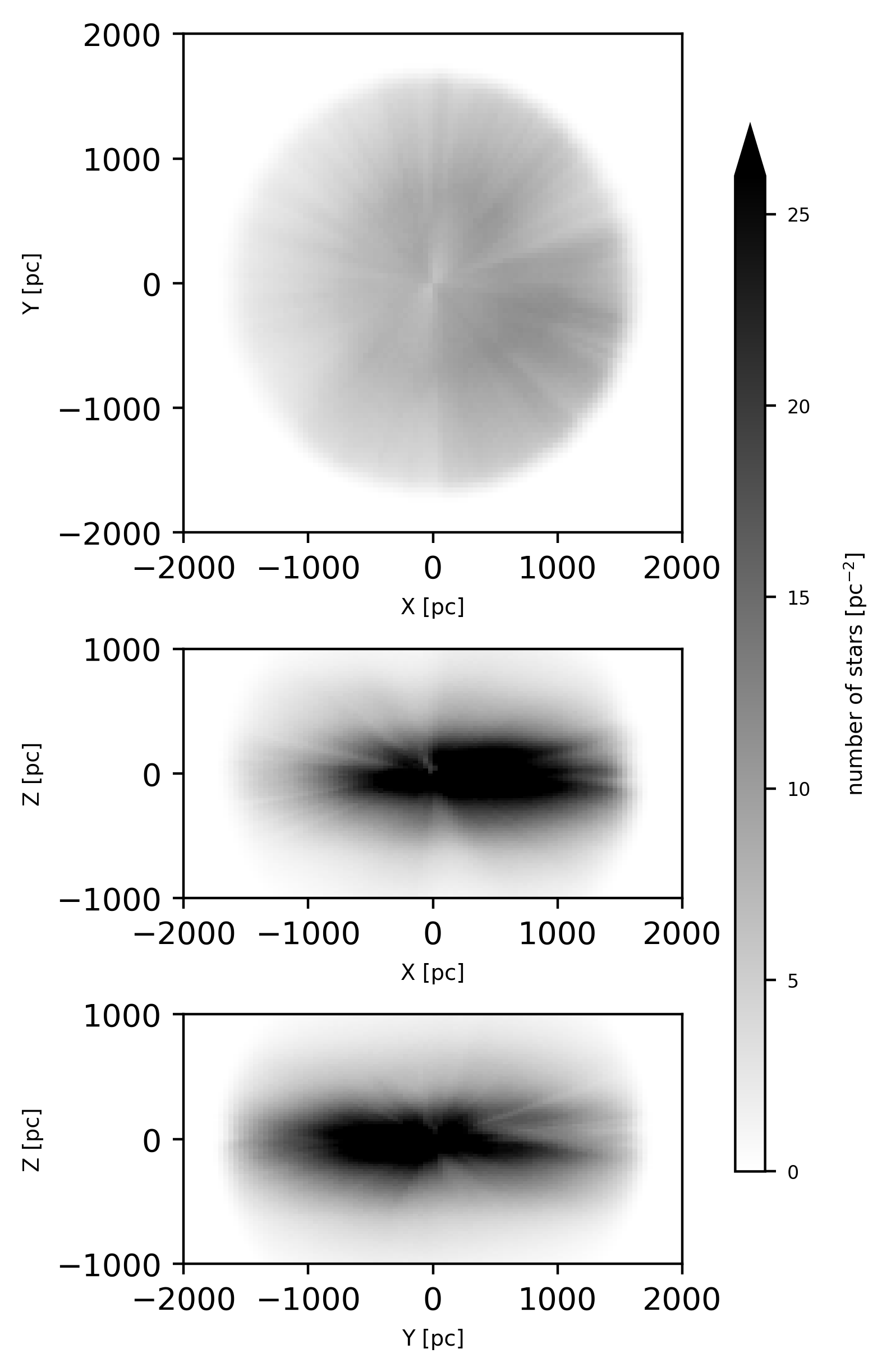
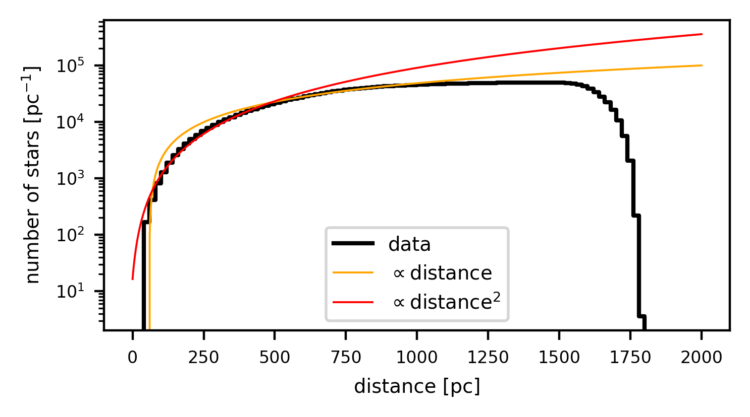
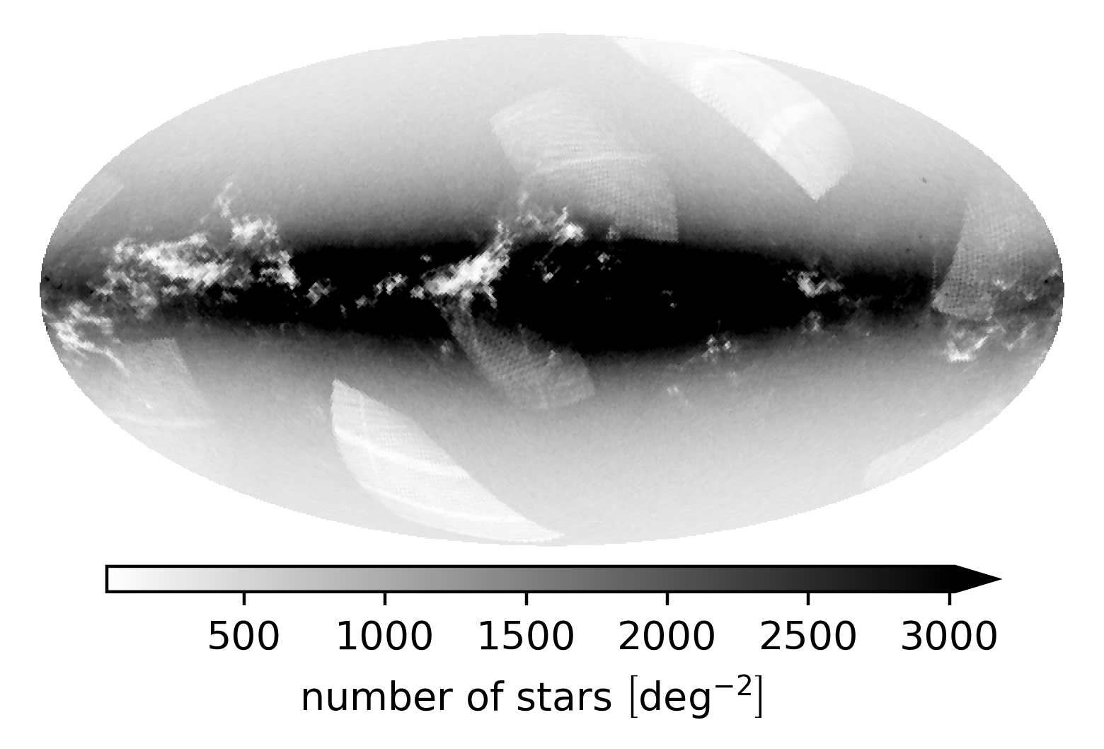
The reliability of our reconstruction is predominantly limited by the quality and quantity of the data. Both strongly depend on the POS position and distance. \Cref{fig:density_of_stars} shows 2D histograms of stellar density in heliocentric Galactic Cartesian (X, Y, Z) projections, as well as the number of stars as a function of distance. The densities of stars per distance bin first increases approximately quadratically with distance before falling off to a linear increase. At approximately $1.5\,\hbox{kpc}$ the number of stars per distance bin levels off before we start deselecting stars by requiring that they have a >1 sigma chance of being within 1.8kpc in distance. \Cref{fig:density_of_stars_mollview} shows a POS histogram of the stars. A clear imprint of the Gaia BP/RP selection function is visible, cf. CantatGaudin2022. A systematic undersampling of stars behind dense dust clouds is also apparent. We expect our reconstruction to be more trustworthy in regions of higher stellar density. Due to the obscuring effect of dust, regions within and behind dense dust clouds should be treated with more caution.
Heliocentric Galactic Cartesian (X, Y, Z) projected histograms.
 }}
}
}}
}
Number of stars as a function of distance.
 }}
}
\caption{%
2D histograms of the density of stars in heliocentric Galactic Cartesian (X, Y, Z) projections, as well as the density of stars as a function of distance, for the subset of the ZGR23 catalog used in the reconstruction of our 3D dust map.
The latter visualization additionally shows a linear growth and a quadratic growth with distance for comparison.
}
}}
}
\caption{%
2D histograms of the density of stars in heliocentric Galactic Cartesian (X, Y, Z) projections, as well as the density of stars as a function of distance, for the subset of the ZGR23 catalog used in the reconstruction of our 3D dust map.
The latter visualization additionally shows a linear growth and a quadratic growth with distance for comparison.
}
 }}
\caption{%
Plane-of-sky distribution of the subset of ZGR23 stars used in the reconstruction of our 3D dust map.
}
}}
\caption{%
Plane-of-sky distribution of the subset of ZGR23 stars used in the reconstruction of our 3D dust map.
}
3. Priors
Our quantity of interest is the 3D distribution of differential ZGR23 extinction $\rho$.\footnotemark By definition the differential extinction is positive. Furthermore, we assume it to be spatially smooth. A priori we assume the level of smoothness to be spatially stationary and isotropic.
The ZGR23 extinction is in arbitrary units but can be translated to an extinction at any given wavelength by using the extinction curve published at https://doi.org/10.5281/zenodo.6674521. Furthermore, dust extinction can be translated to a rough hydrogen volume density by assuming a constant extinction to hydrogen column density ratio (see e.g. Zucker2021). }
To reconstruct the 3D volume efficiently, we discretize it in spherical coordinates. Specifically, we discretize our reconstructed volume into HEALPix spheres at logarithmically spaced distances. We adopt an $N_\text{side}$ of $256$, corresponding to $786,432$ POS bins. This $N_\text{side}$ corresponds to an angular resolution of $14'$.\footnotemark For the LOS direction, we adopt $772$ logarithmically spaced distance bins of which $256$ are used for padding. In contrast to reconstructions with linearly-spaced voxels in distance, we are able to probe much larger volumes while maintaining high resolution at nearby distances.
The angular resolution of $14'$ refers to the angular size of our voxels. It provides a lower bound on the minimum separation between dust structures that we are able to resolve. In practice the resolution is highly position dependent and is predominantly driven by the quantity and quality of the data. }
We encode both positivity and smoothness in our model by assuming the differential extinction to be log-normally distributed
with normally distributed $s$, where $s$ is drawn from a Gaussian process with homogeneous and isotropic correlation kernel $k$. From previous reconstructions of the differential extinction for the Gaia DR2 G-band $A_G$ (Leike2020), we have constraints on the correlation kernel of the logarithm of the differential extinction in a volume around the Sun ($|X| < 370pc,, |Y| < 370pc,, |Z| < 270\,\hbox{pc}$). As part of our prior model we use the inferred $A_G$ extinction kernel from Leike2020. To account for the conversion between the ZGR23 extinction and $A_G$ extinction, we add a global multiplicative factor to $s$ in our model.\footnotemark Furthermore, we infer an additive offset in the differential extinction. We place a log-normal prior on the multiplicative parameter and a normal prior on the additive one
By doing so (and by using ZGR23) we implicitly assume a spatially stationary reddening law for dust. }
We enforce the correlation kernel $k$ using Iterative Charted Refinement (ICR) (Edenhofer2022). ICR enables us to enforce a kernel on arbitrarily spaced voxels by representing the modeled volume at multiple resolutions. It starts from a very coarse view of our modeled volume. On this coarsest scale, ICR models the GP with learned voxel excitations $\xi_e^{(0)}$ and an explicit full kernel covariance matrix. A priori the parameters $\xi_e^{(0)}$ are standard normally distributed and coupled according to $k$ via ICR. It then iteratively refines $n_\text{lvl}$ times its coarse view of the space with local, fine, a priori standard normally distributed corrections $\xi_e^{(1)},\dots,\xi_e^{(n_\text{lvl})}$ until reaching the desired resolution. In each refinement it uses $n_\mathrm{csz}$ neighbors from the previous refinement to refine one coarse pixel into $n_\mathrm{fsz}$ fine pixels. See \Cref{alg:icr}.
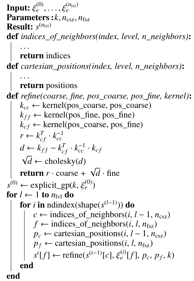
Pseudocode for ICR creating a GP $s$ from uncorrelated excitations $\left\{ \xi_e^{(0)},\dots,\xi_e^{(n_\mathrm{lvl})} \right\}$.
Each coarse pixel at location $j$ is iteratively refined to $n_\mathrm{fsz}$ fine pixels using $n_\mathrm{csz}$ coarse pixel neighbors.
The correlation kernel is denoted by $k$.
Square brackets after variables and the two functions ndindex and shape denote NumPy-like (Harris2020) indexing routines.
The call explicit\_gp refers to an unspecified Gaussian Process model explicitly representing the covariance of $k$ for the pixel positions modeled by $\xi^{(0)}_e$.
}
ICR uses local corrections at varying resolutions and within a refinement assumes the previous iteration to have modeled the GP without error. Both lead to slight errors in representing the kernel. For our use case we encounter errors in representing the kernel of a few percent. We accept these errors as a trade-off that enables the reconstruction to probe larger volumes. We refer to Edenhofer2022 for a detailed discussion of the kernel approximation errors.
Overall, our model for the prior reads
where we denote the learned multiplicative scaling of $s$ by $\mathrm{scl}$, the learned additive offset by $\mathrm{off}$, and re-expressed both in terms of a priori standard normally distributed parameters $\xi_\mathrm{scl}$ and $\xi_\mathrm{off}$ respectively. The act of expressing $\mathrm{scl}$, $\mathrm{off}$ and $s$ via parameters with an a priori simpler distribution, here a standard normal distribution, is called re-parameterization. See Rezende2015 for a detailed discussion on this subject.
4. Likelihood
To construct the likelihood we first need to define how the differential extinction $\rho$ --- our quantity of interest --- connects to the measured data $\mathcal{D}$. Our data comprises POS position, extinction $\mathcal{D}_A$, and parallax $\mathcal{D}_\omega$ data. The POS position is in essence without error. The extinction data $\mathcal{D}_A=\{A,\sigma_A\}$ is in the form of integrated LOS extinctions to stars $A$ and associated uncertainties $\sigma_A$ The parallax data $\mathcal{D}_\omega=\{\omega, \sigma_\omega\}$ similarly is in the form of parallax estimates $\omega$ and uncertainties $\sigma_\omega$.
In our model, we focus on the measured extinction $A$ and do not predict parallaxes to stars. Instead, we condition our model on the parallax data $\mathcal{D}_\omega$ and split the likelihood into the probability of the measured extinction given the true extinction $a$ and the probability of the true extinction given uncertain parallax information
The first term of the integrand is constrained by the quality of the extinction measurements and the second by the quality of the parallax measurements.
4.1 Response
The second term in \Cref{eq:top_level_likelihood} $P(a,|,\rho,\mathcal{D}_\omega)$ can be expressed as the joint probability of extinction and true distance $d$ marginalized over the true distance
We neglect data selection effects, i.e. $a$'s dependence on $\mathcal{D}_\omega$ given $d$ and $d$'s dependence on $\rho$ given $\mathcal{D}_\omega$, and use that the true extinction $a$ at known distance $d$ is simply the LOS integral of $\rho$ along the LOS to the star from zero to $d$
with $\rho[\mathrm{POS}]$ the slice of $\rho$ at the POS positions of the stars, $\delta$ the Dirac delta distribution defined by $\int_{-\infty}^{\infty}\mathrm{d}x\ f(x)\delta(x)=f(0)$ for any continuous $f$ with compact support, and $R$ the response which maps from $\rho$ to the domain of the measured extinction.
We approximate $P(a|\rho,\mathcal{D}_\omega)$ with a normal distribution
with mean $\bar{a}$ and standard deviation $\sigma_a$ to obtain a tractable expression for \Cref{eq:top_level_likelihood}. The mean extinction $\bar{a}$ is
Assuming the parallax ${1}/{d}$ is normally distributed, i.e. $P(d|\mathcal{D}_\omega)=\mathcal{G}\left({1}/{d} \vert \omega, \sigma_\omega^2\right)$ with mean $\omega$ and standard deviation $\sigma_\omega$, then
with $\mathrm{sf}_\mathcal{G}\left({1}/{d} \vert \omega, \sigma_\omega^2\right) := 1 - \int_{-\infty}^{{1}/{d}}\mathrm{d}\omega'\ \mathcal{G}\left(\omega' \vert \omega, \sigma_\omega^2\right)$ the survival function of the normal distributed parallax.
The standard deviation $\sigma_{a}$ can be understood as an additional error contribution for marginalizing over the distance. The error depends on the distance uncertainty and the dust along the full LOS
Evaluating both $\bar{a}$ and $\sigma_a^2$ is comparatively cheap in a spherical coordinate system since for a discretized sphere $R^{d}(\rho)$ is simply the cumulative sum of $\rho$ along the distance axis weighted by the radial extent of each voxel.
4.2 Likelihood and Joint Probability Density
We assume the measured extinction to be normally distributed around the true extinction $a$. We take the inferred extinction $A$ from the catalog to be the mean of the normal distribution. The accompanying uncertainty $\sigma_A$ in the catalog is assumed to be the standard deviation of $P(A,|,a)$.
Some stars will have underestimated uncertainties either due to mismodeled intrinsic stellar properties in the inference or bad photometric measurements that were not flagged. We want our model to be able to detect and deselect stars which are in strong disagreement with the rest of the reconstruction. We do so by inferring an additional multiplicative factor per star $n_\sigma$ which scales $\sigma_A$. A priori, we assume $n_\sigma$ to be drawn from a heavy-tailed distribution. Specially, we assume $n_\sigma$ to follow an inverse gamma distributed. We again express $n_\sigma$ in terms of standard normally distributed parameters $n_\sigma(\xi_\sigma)$ in the inference.
To summarize, our approximate likelihood first introduced in \Cref{eq:top_level_likelihood}, reads
The uncertainty in the extinction $\sigma_{A}$ is scaled by $n_\sigma$ to deselect outliers and increased by $\sigma_{a}^2$ due to marginalizing over the distance uncertainty.
The joint probability density function of data and parameters reads
with $\xi$ the vector of all parameters of the model $\left\{\xi_e^{(0)},\dots,\xi_e^{(n_\mathrm{lvl})},\xi_\mathrm{scl},\xi_\mathrm{off},\xi_\sigma\right\}$. The complexity of the prior distributions has been fully absorbed into the transformations $s(\xi)$, $\mathrm{scl}(\xi)$, $\mathrm{off}(\xi)$, and $n_\sigma(\xi)$ from the a priori standard normally distributed parameters $\xi$.
Parameters of the prior distributions. The parameters $s$, $\mathrm{scl}$, and $\mathrm{off}$ fully determine $\rho$. They are jointly chosen to a prior yield the kernel reconstructed in Leike2020.
| Name | Distribution | Mean | Standard Deviation | Degrees of Freedom |
|---|---|---|---|---|
| s | Normal | 0.0 | Kernel from Leike2020 | 786,432 × 772 |
| scl | Log-Normal | 1.0 | 0.5 | 1 |
| off | Normal | $-6.91\left(\approx\ln10^{-3}\right)$ prior median extinction from Leike2020 |
1.0 | 1 |
| Shape Parameter | Scale Parameter | |||
| $n_\sigma$ | Inverse Gamma | 3.0 | 4.0 | #Stars = 53,880,655 |
Our priors in terms of non-standard-normal parameters are summarized in \Cref{tab:priors}. The priors for $s$, $\mathrm{scl}$, and $\mathrm{off}$ are chosen to a priori yield the kernel reconstructed in Leike2020. In contrast to Leike2020, we do not learn a full non-parametric kernel. However, we do infer $\mathrm{scl}$ and $\mathrm{off}$, the scale and zero-mode of the kernel. The prior for $n_\sigma$ is chosen such that the inverse gamma distribution has mode $1$ and standard deviation $2$.
5. Posterior Inference
In the previous section we took special care to express our model not only in terms of physical parameters, like the differential extinction density $\rho$, but also in terms of more simple parameters $\xi$. The act of expressing the parameters of the model $\mathrm{scl}$, $\mathrm{off}$, $s$, and $n_\sigma$ in terms of a priori standard normal distributed variables $\xi$ is called standardization, a special from of re-parameterization (see Rezende2015). Effectively we are shifting complexity from the prior to the likelihood. However, both the non-standardized and the standardized formulation of the joint model are equivalent. Standardizing models can lead to better conditioned inference problems as the parameters all vary on the same scales --- if the prior is not in conflict with the likelihood. We are going to use an inference scheme that relies on the standardized formulation.
We want to infer the posterior for our standardized model from \Cref{eq:joint_model}. Directly probing the posterior via sampling methods like Hamiltonian Monte Carlo Hoffman2011 is computationally infeasible. Instead, we use variational inference to approximate the true posterior. Specifically, we use Metric Gaussian Variational Inference (MGVI, Knollmueller2019). We summarize the main idea behind MGVI in \Cref{appx:mgvi}. We do not approximate the posterior of the noise inference parameter $n_\sigma(\xi_\sigma)$ via variational inference and instead use only the maximum of the posterior for $\xi_\sigma$.
To speed up the inference, we start the reconstruction at a lower resolution ($196,608$ POS bins at $N_\text{side}=128$ and $388$ LOS distance bins) and restrict the inference to a subset of stars with a $\geq 2$ sigma chance of being within 600pc and a $\geq 2$ sigma chance of being farther than 40pc. We successively increase the distance range of the map up to which stars are incorporated in steps of 300pc from 600pc to 1.8kpc. Every time we increase the distance range, we reset the parameters for $n_\sigma$. Then, after all data is incorporated, we increase the angular and distance resolution of the reconstruction to the final resolution.
Our data selection deselects stars close to the maximum distance probed (c.f. \Cref{fig:density_of_stars}). This effect leads to the outer regions of the map being informed by relatively fewer stars compared to the inner regions. We observe that these regions are prone to producing spurious features. For our final data products we remove the outermost 550pc from the data constrained volume as we observe artifacts aligned with our data incrementation strategy within these regions. We believe 550pc to be a conservative cut but we advise caution when finding structures perfectly aligned with a sphere around the sun at 600pc, 900pc, or 1200pc.
ZGR23 assumes all extinctions to be strictly positive. We neglect this constraint by assuming Gaussian errors which leads to an artificial spike in extinction in the first few voxels in each direction. As we know those regions to be effectively free of dust from previous reconstructions c.f. Leike2020, we remove the innermost HEALPix spheres until the mean POS differential extinction as a function of distance reaches a local minimum at 69pc. We release an additional HEALPix map of integrated extinction out to 69pc from the sun to correct integrated LOS predictions for the removed extinction.
Our inference heavily utilizes derivatives of various components of our model. Derivatives are used for the minimization as well as for the variational approximation of the posterior. Previous models such as Leike2019, Leike2020 relied on the Numerical Information Field Theory (NIFTy) package (Selig2013, Steiniger2017, Arras2019) and were limited to running on CPUs.
We employ a new framework called NIFTy.re (Edenhofer2023NIFTyRE) for deploying NIFTy models to GPUs. NIFTy.re is part of the NIFTy Python package and internally uses JAX (Jax2018) to run models on the GPU. We are able to speed up the evaluation of the value and gradient of \Cref{eq:joint_model} by two orders of magnitude by transitioning from CPUs to GPUs. Our reconstruction ran on a single NVIDIA A100 GPU with 80 GB of memory for about four weeks.
6. Caveats
We believe statistical uncertainties are the dominant source of uncertainty for our reconstruction. However, it is important to also consider sources of systematic uncertainties. Depending on the application, the systematic uncertainties may be more important than the statistical uncertainties. The data that informed the reconstruction, the model with which we inferred it, and the inference procedure all contribute to the model systematic uncertainties.
Naturally, the data themselves is a source of systematic uncertainties (spatially stationary reddening law, mismodeling of binaries, etc., see Zhang2023) and additionally is known to be incomplete. Given lower stellar densities in heavily obscured regions, volumes of the map behind dense dust clouds are poorly constrained by the data and limits the map's fidelity, c.f. \Cref{fig:density_of_stars_mollview}. Thus, we believe our dust reconstruction to be an underestimation of the true extinction toward dense dust clouds. Zucker2021 also note this effect when comparing the Leike2020 map with 2D integrated extinction maps based on infrared photometry, finding that the Leike2020 is not sensitive to regions with $A_V \gtrsim 2$ mag.
Our model includes a number of approximations. First, we assume a GP-prior on the logarithmic dust extinction using the kernel from Leike2020 and additionally only apply it approximately via ICR. Second, we assume $\mathcal{D}_\omega$ to be independent of $\mathcal{D}_A$. Third, we assume the parallax error to be Gaussian, and fourth, we assume the extinction error to be Gaussian.
For extremely low extinctions the assumption of $A$ being Gaussian is poor due to the positivity prior in the ZGR23 catalog. We correct for this bias towards higher estimated extinction in regions with assumed extremely low true extinctions post-hoc by cutting away the innermost 69pc as described in \Cref{sec:posterior_inference} and publish an auxiliary map of integrated extinction out to 69pc from the sun to correct integrated LOS predictions for the removed extinction.
We further release a catalog of the predicted extinctions of our model to all stars that we use for the reconstruction to allow for additional validation work. In \Cref{appx:extinction_catalog}, we perform a non-exhaustive comparison of our predictions versus the ZGR23 ones. We find that both predictions for the extinction to stars disagree below 50 mmag and above 4 mag (34% more stars than expected have larger respectively smaller extinction prediction compared to ZGR23). See \Cref{appx:extinction_catalog} for more details.
Furthermore, our posterior inference is an approximation. We assume our approximation of the true posterior accurately captures the intrinsic model uncertainties c.f. (Arras2022, Leike2019, Leike2020, Mertsch2023, Roth2023DirectionDependentCalibration, Hutschenreuter2023, Tsouros2023, Roth2023FastCadenceHighContrastImaging, Hutschenreuter2022). However, we do need to worry about structures getting burned in when we increase the maximum distance probed during the inference from 600 pc to 1800 pc in steps of 300pc as described in \Cref{sec:posterior_inference}. We check the final reconstruction for this effect by comparing it against a larger reconstruction which does not subselect the stars based on their distance during the inference but uses only a small sub-sample of ZGR23 stars with more stringent quality flags. The larger reconstruction which extends out to 2kpc in distance is released as an additional data product. We find no significant differences between both runs. See \Cref{appx:2kpc_reconstruction} for details on the larger reconstruction.
7. Results
We reconstruct 12 samples (6 antithetically drawn samples) of the 3D dust extinction distribution which each encompasses 607,125,504 differential extinction voxels.
The voxels are arranged on $772$ HEALPix spheres with $N_\text{side}=256$ spaced at logarithmically increasing distances.
After removing the innermost <69pc and outermost >1250pc HEALPix spheres, we are left with $516$ HEALPix spheres.
The samples and the posterior mean for the reconstruction are publicly available at https://doi.org/10.5281/zenodo.8187943.
We also provide the posterior mean and standard deviation of the reconstruction interpolated to heliocentric Galactic Cartesian Coordinates (X, Y, Z) and Galactic spherical Coordinates ($l$, $b$, $d$) as well as the scripts for the interpolation.
Furthermore, the map can be queried via the dustmaps Python package (Green2018Dustmaps).
See \Cref{appx:using_the_reconstruction} for further details on using the reconstruction.
The distance resolution in our reconstruction is highest for close-by voxels and decreases further out. Our highest distance resolution is 0.4pc and our lowest distance resolution is 7pc.\footnotemark Our angular resolution is $14'$ and is independent of the distance.
The stated highest respectively lowest distance resolutions of 0.4pc respectively 7pc refer to the minimum respectively maximum extent of the voxels in the radial direction. This is not necessarily the same as the minimum separation in distance at which we are able to resolve structures with the given data and our model. In practice the resolution is highly position dependent and is predominantly driven by the quantity and quality of the data. }
The reconstruction is in terms of the unitless ZGR23 extinction as defined in Zhang2023. For visualization purposes we translate the ZGR23 extinction to Johnson's V-band $\lambda=540.0{nm}$, i.e., $A_V := A(V=540.0{nm})$. To perform the conversion, we adopt the extinction curve published in ZGR23, and multiply the unitless ZGR23 extinction by a factor of $2.8$. We refer readers to the full extinction curve at https://doi.org/10.5281/zenodo.6674521 from Zhang2023 for the coefficients needed to translate the extinction to other bands.
 }}
\caption{%
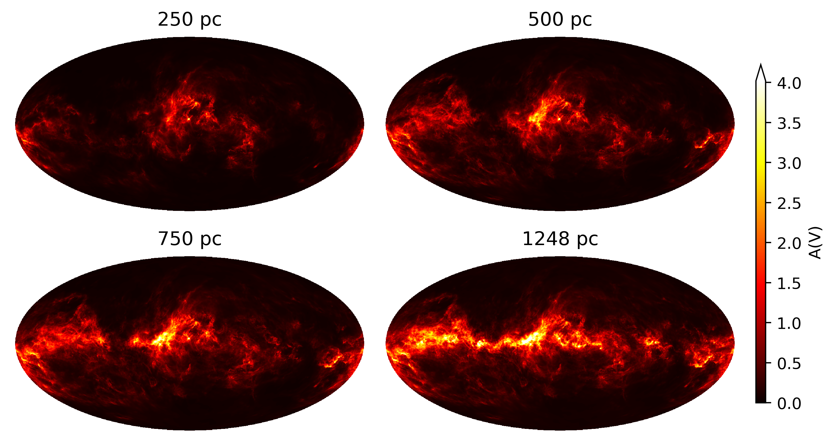
Mollweide projection of the POS integrated $A_V$ extinction out to 250pc, 500pc, 750pc, and up to the maximum distance of our map.
The colorbar saturates at the $99.9%$ quantile.
}
}}
\caption{%
Mollweide projection of the POS integrated $A_V$ extinction out to 250pc, 500pc, 750pc, and up to the maximum distance of our map.
The colorbar saturates at the $99.9%$ quantile.
}
 }}
\caption{%
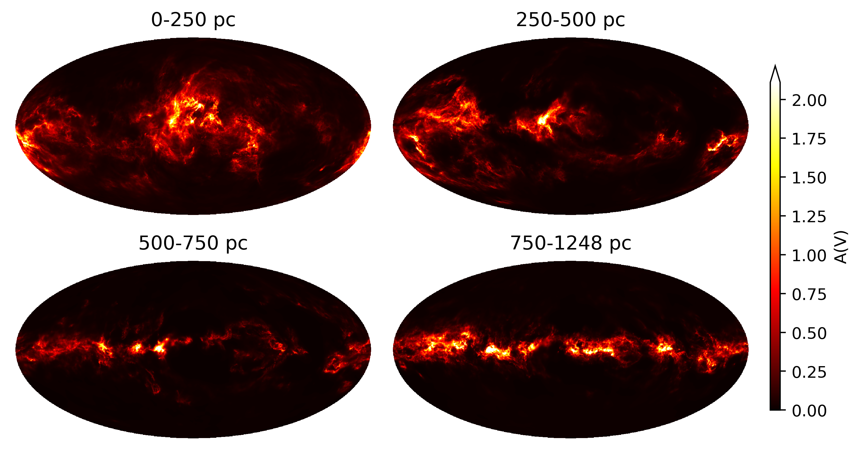
Same as \Cref{fig:integrated_mollview} but showing the difference between the integrated extinctions in between distance slices projection on the POS.
The colorbar saturates at the $99.9%$ quantile.
}
}}
\caption{%
Same as \Cref{fig:integrated_mollview} but showing the difference between the integrated extinctions in between distance slices projection on the POS.
The colorbar saturates at the $99.9%$ quantile.
}
\Cref{fig:integrated_mollview} depicts the POS projection of the posterior mean reconstruction integrated out to 250pc, 500pc, 750pc, and up to the end of our sphere. The $A_V$ values are in units of magnitudes. We see that higher-latitude features like the Aquila Rift are comparatively close-by while structures in the Galactic plane appear only gradually. \Cref{fig:diff_mollview} shows the difference between the integrated POS projections. We recover well known features of integrated dust but are now able to de-project them.
 }}
\caption{%
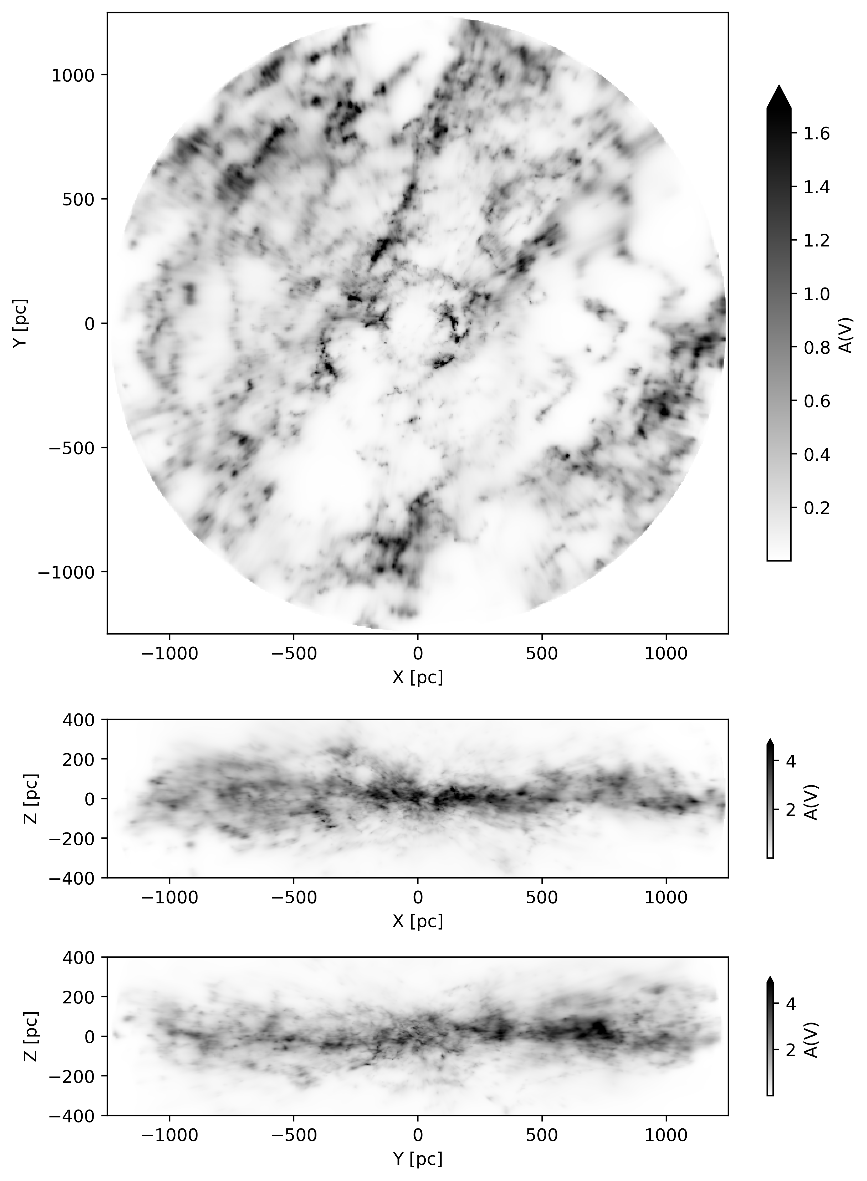
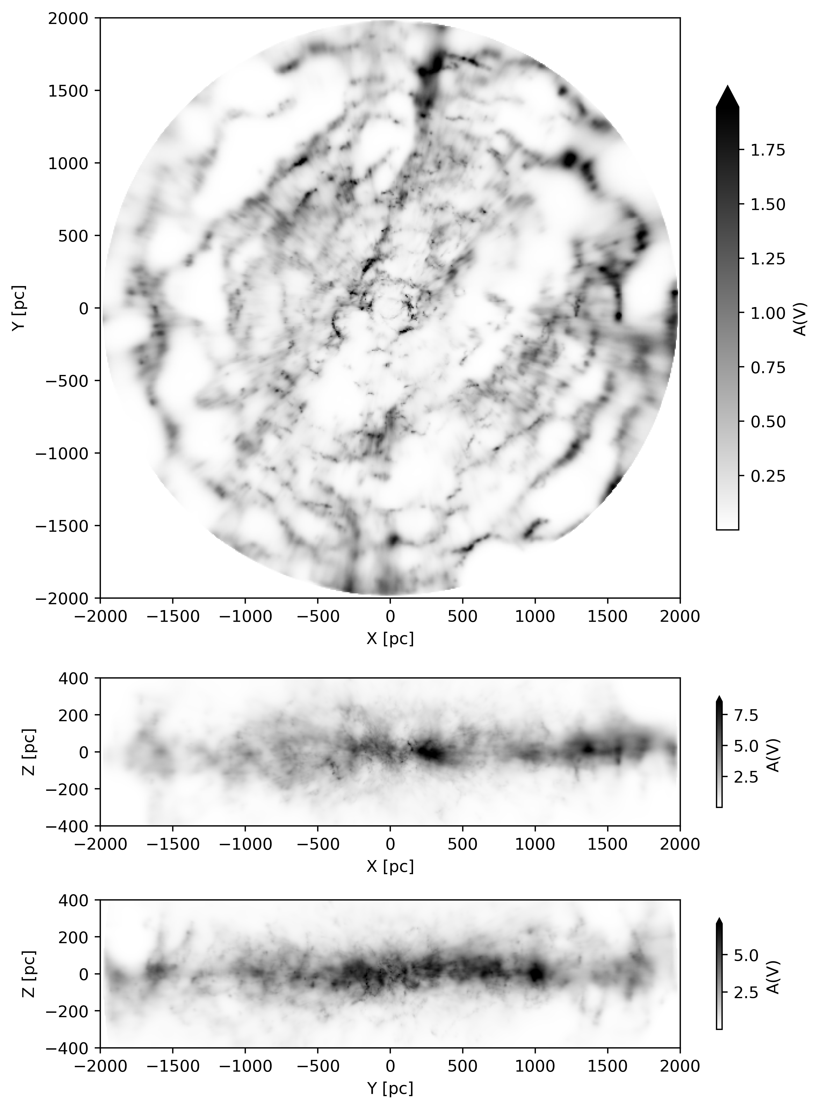
Heliocentric Galactic Cartesian (X, Y, Z) projections of the posterior mean of our 3D dust map in a box with dimensions $2.5kpc \times 2.5kpc \times 0.8\,\hbox{kpc}$ centered on the Sun.
The colorbar is linear and saturates at the $99.9%$ quantile.
A GIF of the posterior samples is shown at https://faun.rc.fas.harvard.edu/gedenhofer/perm/E+23/21b9_final.gif.
A low-resolution 3D interactive version of this figure is available https://faun.rc.fas.harvard.edu/czucker/Paper_Figures/3D_Dust_Edenhofer2023.html.
}
}}
\caption{%
Heliocentric Galactic Cartesian (X, Y, Z) projections of the posterior mean of our 3D dust map in a box with dimensions $2.5kpc \times 2.5kpc \times 0.8\,\hbox{kpc}$ centered on the Sun.
The colorbar is linear and saturates at the $99.9%$ quantile.
A GIF of the posterior samples is shown at https://faun.rc.fas.harvard.edu/gedenhofer/perm/E+23/21b9_final.gif.
A low-resolution 3D interactive version of this figure is available https://faun.rc.fas.harvard.edu/czucker/Paper_Figures/3D_Dust_Edenhofer2023.html.
}
 }}
\caption{%
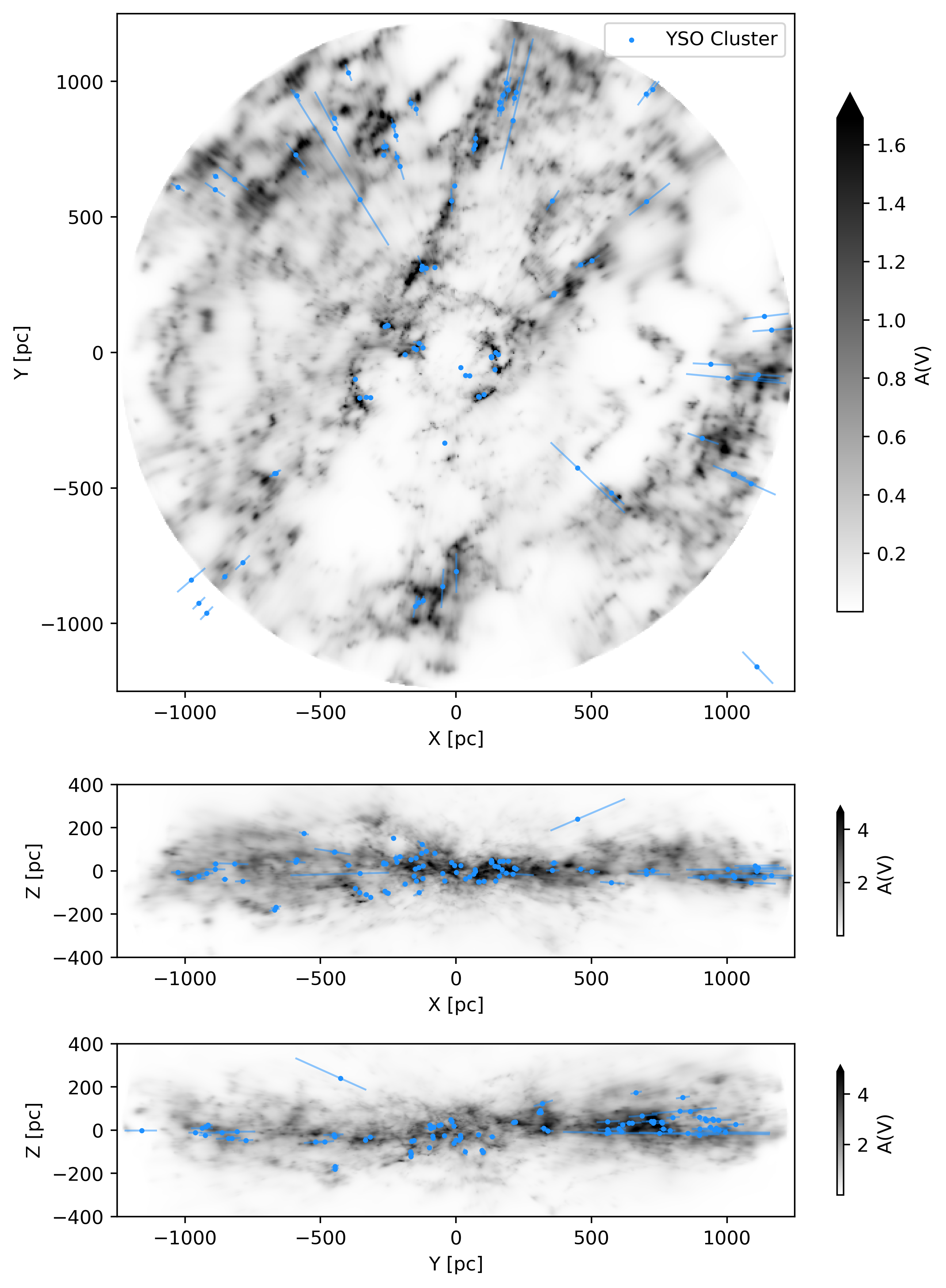
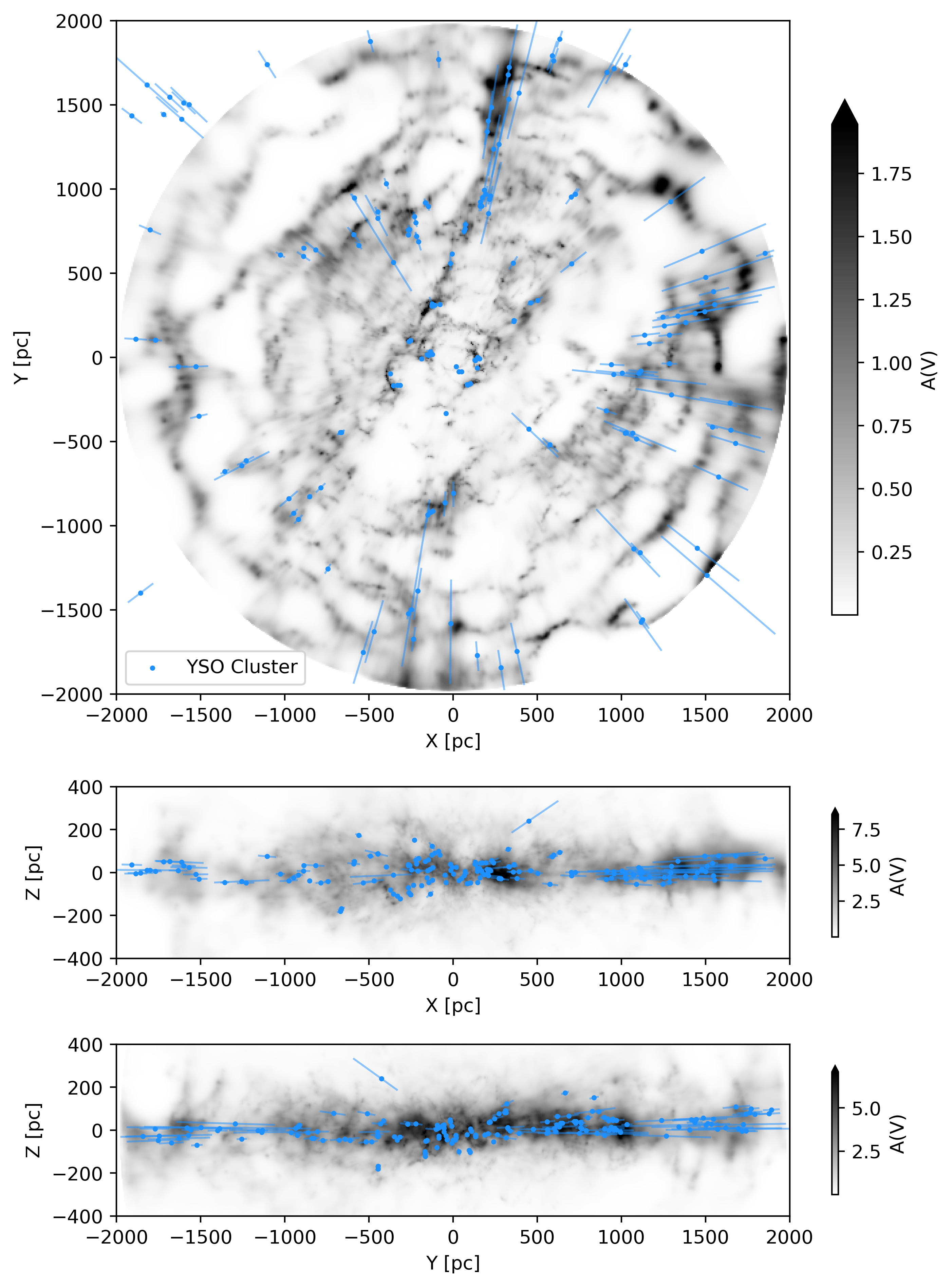
Same as \Cref{fig:galactic} but with a catalog of clusters of young stellar objects (Kuhn2023YSO) based on Kuhn2021, Winston2020, Marton2022 shown as blue dots on top of the reconstruction and their distance uncertainties shown as extended lines.
}
}}
\caption{%
Same as \Cref{fig:galactic} but with a catalog of clusters of young stellar objects (Kuhn2023YSO) based on Kuhn2021, Winston2020, Marton2022 shown as blue dots on top of the reconstruction and their distance uncertainties shown as extended lines.
}
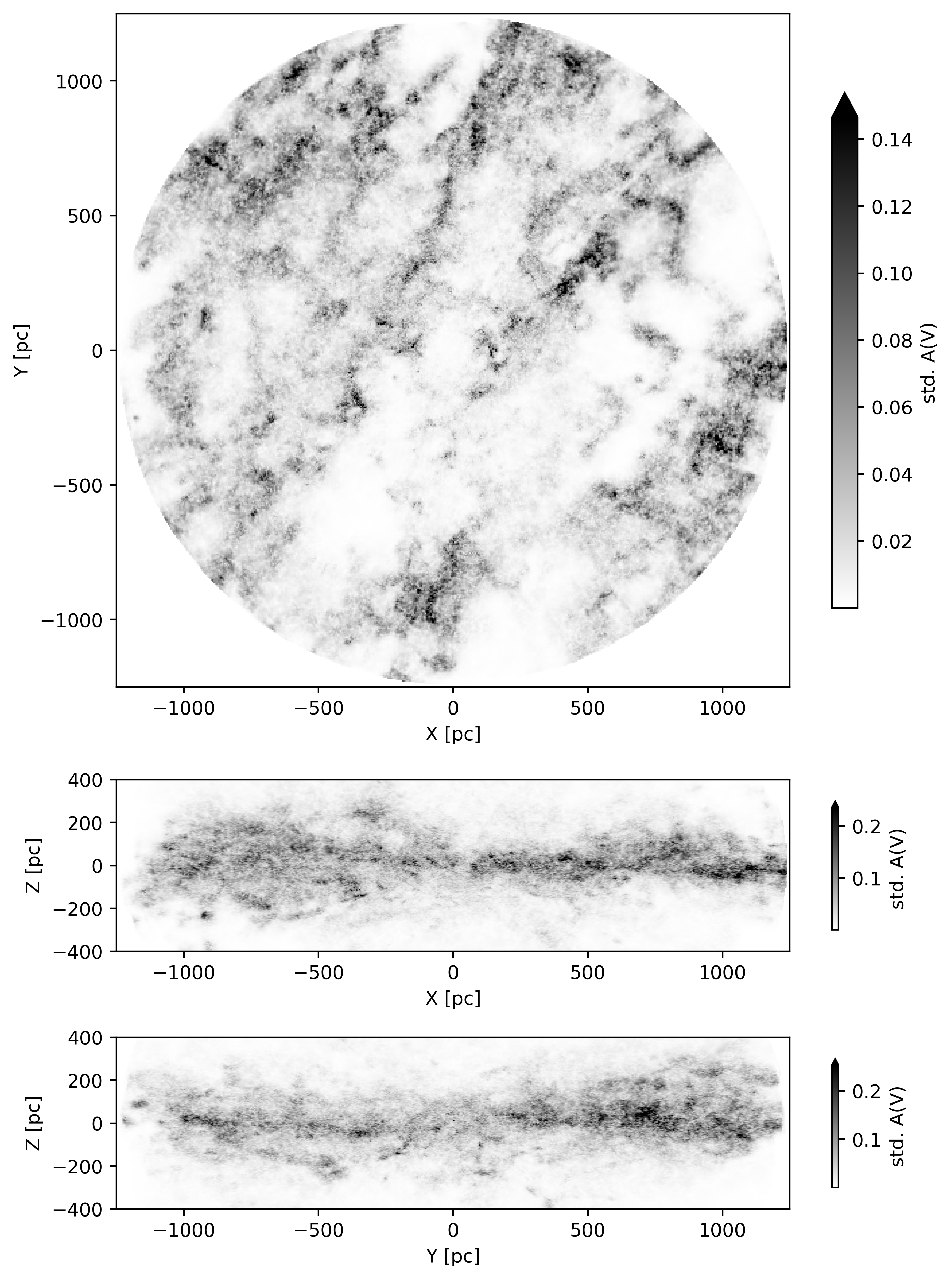 }}
\caption{%
Heliocentric Galactic Cartesian (X, Y, Z) projections of the standard deviation of the reconstructed dust extinction integrated within the box $2.5kpc \times 2.5kpc \times 0.8\,\hbox{kpc}$ centered on the Sun.
The colorbar is linear and saturates at the $99.9%$ quantile.
}
}}
\caption{%
Heliocentric Galactic Cartesian (X, Y, Z) projections of the standard deviation of the reconstructed dust extinction integrated within the box $2.5kpc \times 2.5kpc \times 0.8\,\hbox{kpc}$ centered on the Sun.
The colorbar is linear and saturates at the $99.9%$ quantile.
}
\Cref{fig:galactic} show a bird's eye (X, Y), side-on (X, Z), and (Y, Z) projection of the posterior mean of our reconstruction in heliocentric Galactic Cartesian coordinates. The image depicts the innermost $2.5kpc \times 2.5kpc \times 0.8\,\hbox{kpc}$ around the Sun in $A_V$ extinction integrated over $z$ from -400 pc to 400 pc, $y$ in -1.25 kpc to 1.25 kpc, and $x$ in -1.25 kpc to 1.25 kpc, respectively. In \Cref{fig:galactic_ysos} we overlay a catalog of clusters of Young Stellar Objects (YSOs) (Kuhn2023YSO) based on Kuhn2021, Winston2020, Marton2022, which are shown as blue dots. The positions of the YSO clusters visually agree with the positions of dust clouds within the YSO clusters' reported distance uncertainties. The standard deviation of the reconstruction is shown in \Cref{fig:galactic_std}. It is on the order of $10%$ of the posterior mean and tends to increase with distance.
The reconstruction has a high dynamic range and reveals faint dust lanes in the reconstructed volume. Small approximately spherical cavities are evident throughout the map. The dust clouds in the reconstruction are compact and only weakly elongated radially. Prominent large-scale features, such as the Radcliffe Wave Alves2020 and the Split (Lallement2019), have been resolved at an unprecedented level of detail, previously only accessible for the most nearby dust clouds.
7.1 Comparison to Existing 3D Dust Maps
In this section, we compare our map to other 3D dust maps in the literature. We denote the dust map by Leike2020 by LGE20, Vergely2022 by VLC22, Green2019 by Bayestar19, and Leike2022 by L+22 in this section. For the purposes of comparison, we show the posterior mean. We release the statistical uncertainties as additional data products, and we strongly advise taking into account these statistical uncertainties for any quantitative analysis. However, the differences between the various 3D dust reconstructions discussed here are systematic differences and are not captured by the reconstructed statistical uncertainties.
 }}
\caption{%
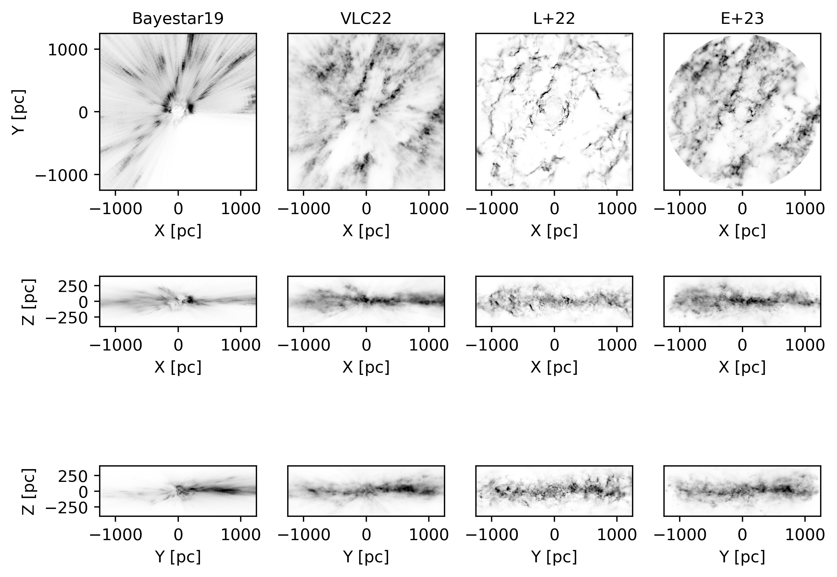
Side-by-side views of the 3D dust maps from Bayestar19, VLC22, L+22 and this work, shown in heliocentric Galactic Cartesian (X, Y, Z) projections.
The colorbars are saturated at the $99.9%$ quantile of the respective reconstruction.
}
}}
\caption{%
Side-by-side views of the 3D dust maps from Bayestar19, VLC22, L+22 and this work, shown in heliocentric Galactic Cartesian (X, Y, Z) projections.
The colorbars are saturated at the $99.9%$ quantile of the respective reconstruction.
}
In \Cref{fig:sidebyside}, we show 3D (X, Y, Z) projections of the maps, comparing Bayestar19, VLC22, and this work side-by-side. All four maps agree on the general structure of the distribution of dust.
This work, L+22, and VLC22 have a comparable distance resolution while Bayestar19 only features comparatively few distance bins and more strongly pronounced fingers-of-god. Compared to L+22, we feature more homogenously extended dust clouds and significantly less radial wiggles in the distances to dust clouds. Compared to VLC22, we feature more compact dust clouds, less grainy structures, and a higher dynamic range. Both this work and VLC22 feature dust clouds in a comparable volume around the sun despite the VLC22 map technically extending out further in Galactic heliocentric X and Y.
 }}
\caption{%
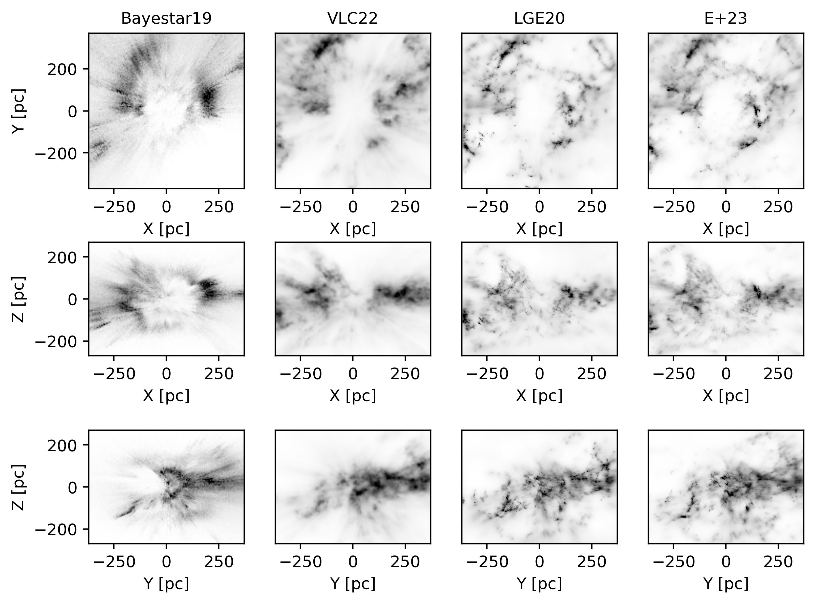
Zoomed-in version of \Cref{fig:sidebyside} for the volume reconstructed in Leike2020, now also showing the LGE20 reconstruction for comparison.
We leave out L+22 from the comparison because the authors explicitly focus on larger volumes and trade strongly pronounced artifacts in the inner couple hundred parsecs for a larger probed volume.
The colorbars are again saturated at the $99.9%$ quantile of the respective reconstruction.
}
}}
\caption{%
Zoomed-in version of \Cref{fig:sidebyside} for the volume reconstructed in Leike2020, now also showing the LGE20 reconstruction for comparison.
We leave out L+22 from the comparison because the authors explicitly focus on larger volumes and trade strongly pronounced artifacts in the inner couple hundred parsecs for a larger probed volume.
The colorbars are again saturated at the $99.9%$ quantile of the respective reconstruction.
}
\Cref{fig:sidebyside_leike2020box} shows the same projections for the volume reconstructed in the LGE20 map and includes the LGE20 map for comparison. The zoom-in highlights the close similarity between this work and the LGE20 map. All larger structures have direct correspondences in the other map, yet the distances to the structures are slightly different. Furthermore, the LGE20 map appears slightly sharper. The model in LGE20 is very similar to ours but uses fewer approximations. LGE20 also uses compiled data (StarHorse DR2, see Anders2019). More work is needed to asses the validity of the sharper features in LGE20 not present in this work. The VLC22 map is in good agreement as well but lower resolution. Bayestar19 poorly resolves distances at the scale of the LGE20 map.
 }}
\caption{%
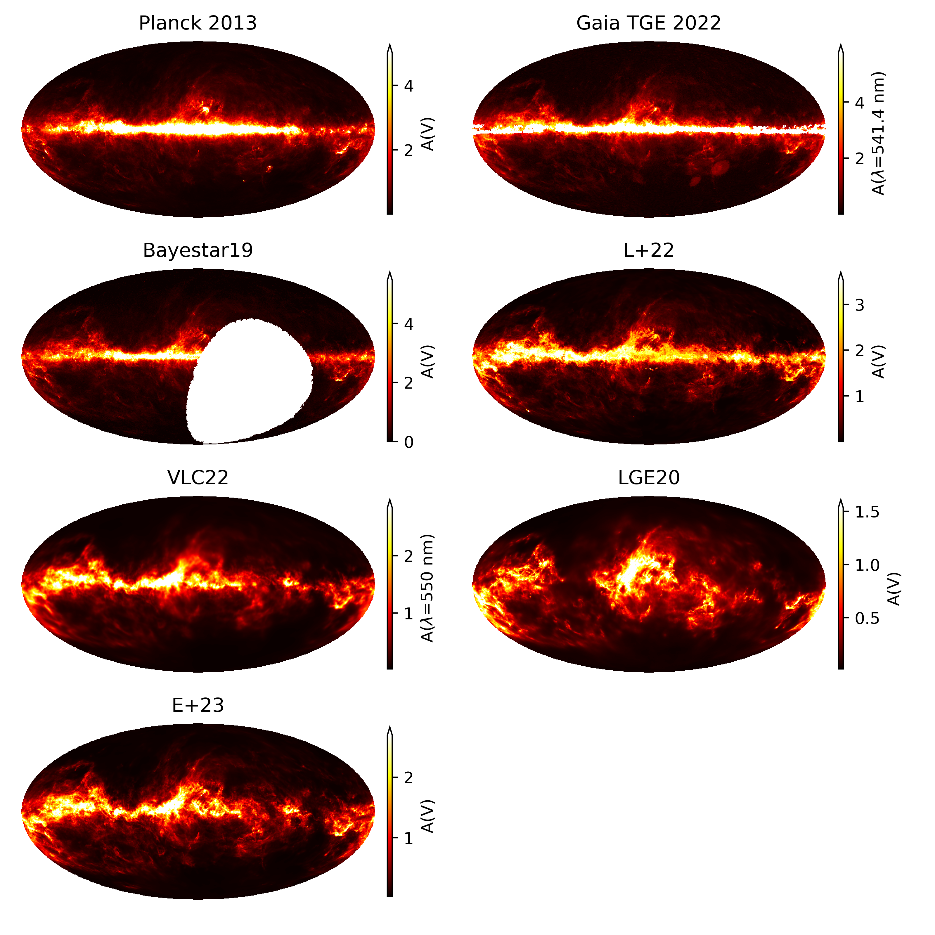
Mollweide projections of total integrated extinction and 3D extinction maps integrated out the maximum distance of the respective map.
Bayestar19 reconstructs up to a maximum distance of 63kpc (maximum reliable distance 10kpc) and is integrated out to that volume.
L+22 reconstructs up to a maximum distance of 16kpc but the authors trust their map only out to 4kpc and we integrate their map only to 4kpc.
VLC22 reconstructs a heliocentric box of size $3kpc \times 3kpc \times 800\,\hbox{pc}$ with $10^3\,\hbox{pc}^3$ voxels with at most $<2.16\,\hbox{kpc}$ in distance and is integrated out to the end of the box.
Likewise, LGE20 reconstructs a heliocentric box of size $\rm |X| < 370pc, |Y| < 370pc, |Z| < 270\,\hbox{pc}$ covering at most $<590\,\hbox{pc}$ in distance and is integrated out to the end of the box.
The colorbars saturate at the respective $99%$ quantile of the map except for the colorbar of Planck 2013 which saturates at 5 mag for better comparability.
}
}}
\caption{%
Mollweide projections of total integrated extinction and 3D extinction maps integrated out the maximum distance of the respective map.
Bayestar19 reconstructs up to a maximum distance of 63kpc (maximum reliable distance 10kpc) and is integrated out to that volume.
L+22 reconstructs up to a maximum distance of 16kpc but the authors trust their map only out to 4kpc and we integrate their map only to 4kpc.
VLC22 reconstructs a heliocentric box of size $3kpc \times 3kpc \times 800\,\hbox{pc}$ with $10^3\,\hbox{pc}^3$ voxels with at most $<2.16\,\hbox{kpc}$ in distance and is integrated out to the end of the box.
Likewise, LGE20 reconstructs a heliocentric box of size $\rm |X| < 370pc, |Y| < 370pc, |Z| < 270\,\hbox{pc}$ covering at most $<590\,\hbox{pc}$ in distance and is integrated out to the end of the box.
The colorbars saturate at the respective $99%$ quantile of the map except for the colorbar of Planck 2013 which saturates at 5 mag for better comparability.
}
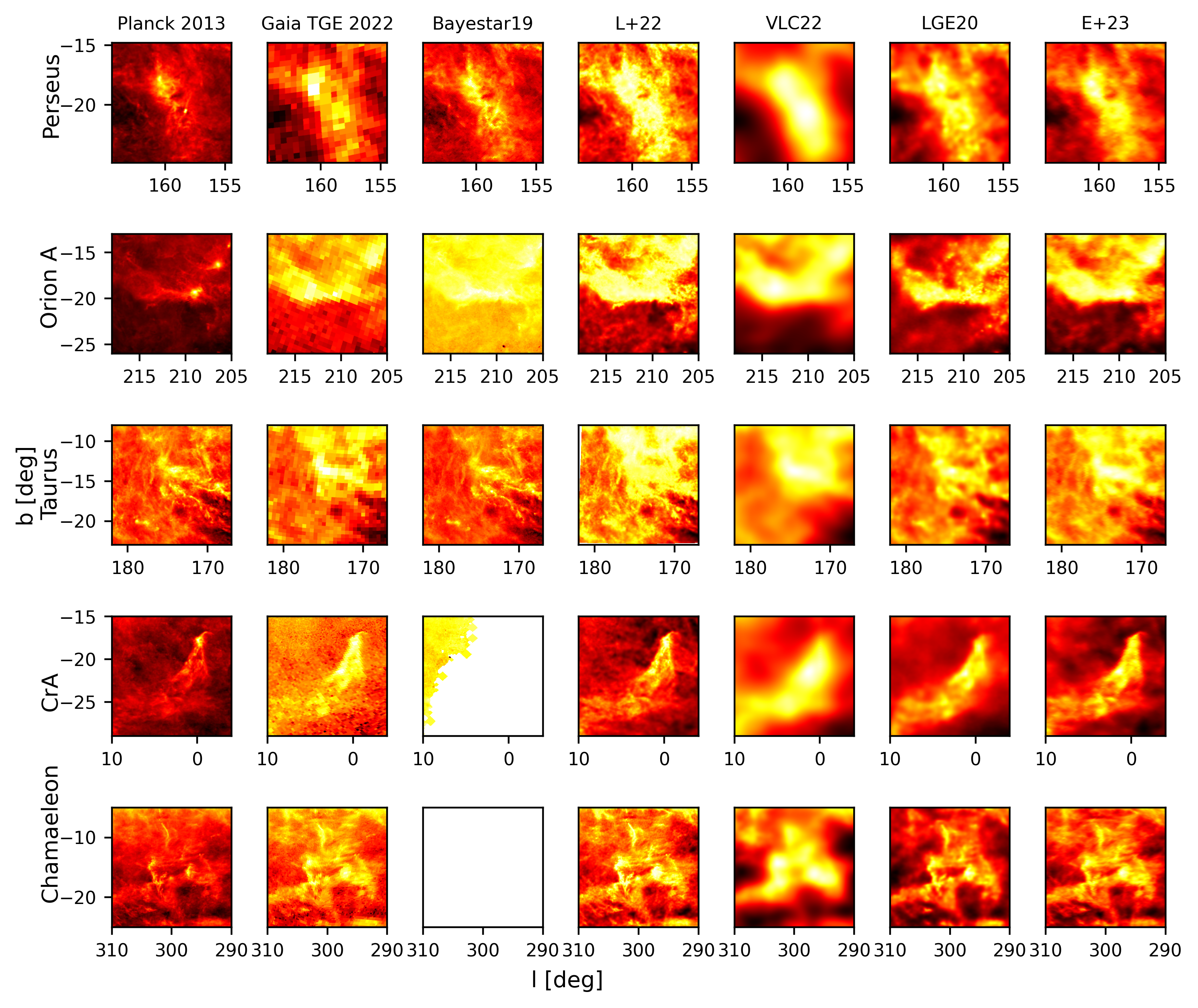
In \Cref{fig:mollview_versus} we compare the POS view of Bayestar19, L+22, VLC22, LGE20 and this work. The respective POS views are integrated out to the maximum distance probed by each map --- $<63\,\hbox{kpc}$ in distance for Bayestar19 (maximum reliable distance 10kpc), $<4\,\hbox{kpc}$ in distance for L+22 (authors trust structures up to 4kpc though the map extends to 16kpc), a heliocentric box of size $3kpc \times 3kpc \times 800\,\hbox{pc}$ with $10^3\,\hbox{pc}^3$ voxels for VLC22 with at most $2.16\,\hbox{kpc}$ in distance, and a heliocentric box of size $\rm |X|, |Y| < 370pc, |Z| < 270\,\hbox{pc}$ and up to $590\,\hbox{pc}$ in distance for LGE20. In addition, we show the Planck 2013 extragalactic dust map (Planck2013) and the Gaia Total Galactic Extinction (TGE) 2022 map (Delchambre2022).
All maps agree on fine structures at high galactic latitudes but differ in the Galactic plane due to the difference in distance up to which the respective reconstruction extends. 3D dust reconstructions do not probe deep enough into the Galactic plane to fully recover the Planck 2013 extragalactic dust map. Bayestar19 and L+22 probe much deeper than VLC22, LGE20 and this work, yet they do not probe the full column of dust seen in Planck 2013 and Gaia TGE 2022. Both VLC22 and our map probe up to a similar depth while LGE20 only probes dust at much closer distances.
 }}
\caption{%
Zoomed-in views toward individual molecular clouds (Perseus, Orion, Taurus, Corona Australis, and Chamaeleon) seen in \Cref{fig:mollview_versus}.
The colorbars are logarithmic and span the full dynamic range of the selected POS slice in every image.
Each row is a separate region and each column a separate reconstruction.
}
}}
\caption{%
Zoomed-in views toward individual molecular clouds (Perseus, Orion, Taurus, Corona Australis, and Chamaeleon) seen in \Cref{fig:mollview_versus}.
The colorbars are logarithmic and span the full dynamic range of the selected POS slice in every image.
Each row is a separate region and each column a separate reconstruction.
}
\Cref{fig:regions_of_interest} shows a zoom-in comparison of the Perseus, Orion A, Taurus, Corona Australis (CrA), and Chamaeleon molecular clouds, integrated out to the maximum distance of each map (4kpc for L+22). Among the 3D dust reconstructions, Bayestar19 and L+22 have arguably the highest angular resolution with 3.4' ($N_\text{side}=1024$) and 1.9' respectively. They resolves the high latitude dust clouds with great detail although L+22 suffers from localized artifacts in patches of the sky. Both LGE20 (1\,\hbox{pc}^3 boxes) and this work ($N_\text{side}=256$) achieve a comparable angular resolution. The VLC22 reconstruction (10^3\,\hbox{pc}^3 voxels) is noticeably lower in resolution and does not resolve the cloud substructure on the POS.
8. Conclusions
We present a 3D dust map with a POS and LOS resolution comparable to Leike2020 that extends out to 1.25kpc.
We use the distance and extinction estimates of Zhang2023 which have much lower extinction uncertainties than competing catalogs while probing a similar number of stars.
Our reconstruction has an angular resolution of $14'$ and a distance resolution of up to 0.4pc.
We show the map to be in good agreement with existing 3D dust maps and improves upon them in terms of covered volume and spatial resolution.
The map is made publicly available at https://doi.org/10.5281/zenodo.8187943 and can also be queried via the dustmaps Python package.
We anticipate that the map will be useful for a wide range of applications in studying the distribution of dust and the ISM more broadly.
We thank Joao Alves for many fruitful discussions at the "Self-Organization Across Scales: From nm to parsec (SOcraSCALES)'' workshop at the Munich Institute for Astro-, Particle and BioPhysics, an institute of the Excellence Cluster ORIGINS in 2022 and afterwards. Furthermore, we thank Jakob Roth for many invaluable discussions about the model and for providing feedback on the early versions of the reconstruction. We thank Alyssa Goodman for providing invaluable feedback on the late versions of the reconstructions. We also thank Michael A. Kuhn for providing us with a unified catalog of Young Stellar Objects. Gordian Edenhofer acknowledges the support of the German Academic Scholarship Foundation in the form of a PhD scholarship ("Promotionsstipendium der Studienstiftung des Deutschen Volkes''). Catherine Zucker acknowledges that support for this work was provided by NASA through the NASA Hubble Fellowship grant #HST-HF2-51498.001 awarded by the Space Telescope Science Institute (STScI), which is operated by the Association of Universities for Research in Astronomy, Inc., for NASA, under contract NAS5-26555. Andrew K. Saydjari acknowledges support by a National Science Foundation Graduate Research Fellowship (DGE-1745303). Andrew K. Saydjari and Douglas Finkbeiner acknowledge support by NASA ADAP grant 80NSSC21K0634 "Knitting Together the Milky Way: An Integrated Model of the Galaxy's Stars, Gas, and Dust''. This work was supported by the National Science Foundation under Cooperative Agreement PHY-2019786 (The NSF AI Institute for Artificial Intelligence and Fundamental Interactions). A portion of this work was enabled by the FASRC Cannon cluster supported by the FAS Division of Science Research Computing Group at Harvard University. We acknowledge support by the Max-Planck Computing and Data Facility (MPCDF). This work has made use of data from the European Space Agency (ESA) mission Gaia (https://www.cosmos.esa.int/gaia), processed by the Gaia Data Processing and Analysis Consortium (DPAC, https://www.cosmos.esa.int/web/gaia/dpac/consortium). Funding for the DPAC has been provided by national institutions, in particular the institutions participating in the Gaia Multilateral Agreement.
9. ZGR23 in dust-free Regions
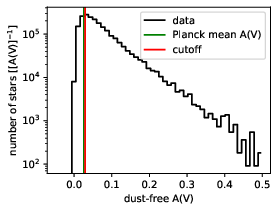
To gauge the reliability of the ZGR23 catalog, we analyze the extinction to stars in dust-free regions, c.f. Leike2019, Leike2020. In dust-free regions, we would expect the extinction to be zero within the uncertainties of the catalog. To classify a region as dust-free, we use the Planck dust emission map (Planck2013). A region is said to be dust-free if the Planck $E(B-V)$ map is below or equal to $0.0095 \mathrm{mag}$ or approximately $0.029$ in terms of $A_V$.
ZGR23 extinction in dust-free regions.
 }}
}
}}
}
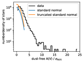
ZGR23 standardized extinction in dust-free regions.
 }}
}
\caption{%
The top plot shows the histogram of the ZGR23 extinctions in dust-free regions translated to $A_V$.
The mean extinction in dust-free regions based on Planck is shown as a vertical green line and the cutoff value translated to $A_V$ for our definition of dust-free is shown in red.
The bottom plot shows the same figure from above, but the extinctions are scaled by their accompanying uncertainties.
A truncated standard normal distribution and a standard normal distribution are plotted on top.
Both ordinates are logarithmic.
}
}}
}
\caption{%
The top plot shows the histogram of the ZGR23 extinctions in dust-free regions translated to $A_V$.
The mean extinction in dust-free regions based on Planck is shown as a vertical green line and the cutoff value translated to $A_V$ for our definition of dust-free is shown in red.
The bottom plot shows the same figure from above, but the extinctions are scaled by their accompanying uncertainties.
A truncated standard normal distribution and a standard normal distribution are plotted on top.
Both ordinates are logarithmic.
}
The first panel of \Cref{fig:zgr23_offset} shows the histogram of ZGR23 extinction to stars with quality_flags<8 in dust-free regions translated to $A_V$.
We see that the histogram of the extinction peaks at the cutoff value and coincides with the mean total extinction as measured by Planck in those regions translated to $A_V$.
The density of extinction values falls of exponentially after the cutoff value.
Overall, the ZGR23 extinction seems to be in good agreement with Planck2013 for dust-free regions.
The second panel of \Cref{fig:zgr23_offset} shows the extinction divided by their uncertainties for the stars from \Cref{fig:zgr23_offset}.
The standardized extinctions are centered around unity, indicating that the ZGR23 extinction indeed are offset from zero by about one standard deviation in dust-free regions.
This is in agreement with the previous finding that the extinctions are centered around the cutoff value instead of clustering around zero.
The width around the center is comparable to a truncated standard normal distribution or a normal distribution.
In total, about $1%$ of the probability mass lies outside the possible range of all ZGR23 extinction with quality_flags<8 if we assume a normal distribution for the extinctions.
Except for outliers far away from the center which can be captured by an outlier model, the ZGR23 catalog seems to be in agreement with POS measurements in dust-free regions and the spread around the cutoff value approximately follows a (truncated) normal distribution. We deem the ZGR23 catalog to be reliable for our purposes and approximate the uncertainties using a normal distribution. We accept the mismodeling of a small fraction of probability mass for a simpler model, see \Cref{sec:caveats,sec:posterior_inference}.
10. Metric Gaussian Variational Inference
The variational inference method Metric Gaussian Variational Inference (MGVI) approximates the true posterior $P(\xi,|,d)$ with a standard normal distribution in a linearly transformed space in which the posterior more closely resembles a standard normal. Let $Q_{\bar{\xi}}(y,|,d)=\mathcal{G}(y(\xi),|,y(\bar{\xi}),\mathbb{1})\left|\frac{\mathrm{d}y}{\mathrm{d}\xi}\right|$ be the approximate posterior and $y(\xi): \xi \mapsto y(\xi)$ the coordinate transformation. In this space the transformed posterior reads $P(\xi(y),|,d)\left|\frac{\mathrm{d}\xi}{\mathrm{d}y}\right|$. We denote the metric of the space in which $P(\xi(y),|,d)\left|\frac{\mathrm{d}\xi}{\mathrm{d}y}\right|$ is "more'' standard normal by $M := \frac{\mathrm{d}y}{\mathrm{d}\xi} \left(\frac{\mathrm{d}y}{\mathrm{d}\xi}\right)^\dagger$. Assuming $y(\xi): \xi \mapsto y(\xi)$ is known, the difficulty lies solely in finding the optimal $\bar{\xi}$ for $Q_{\bar{\xi}}$.
Based on the Fisher information metric and Frequentist statistics, Knollmueller2019 derive a coordinate transformation $y_{\bar{\xi}}(\xi)$ centered on $\bar{\xi}$ that is linear in $\xi$. In Frank2021, the authors find that a set of Riemannian normal coordinates $y_{\bar{\xi}}(\xi)$ centered on $\bar{\xi}$ are an improved, non-linear estimate of the coordinate transform $y(\xi) \approx y_{\bar{\xi}}(\xi)$. The improvements though come at slightly higher computational costs. We refer the reader to Frank2021, Frank2022 for further details on geoVI and its relation to MGVI, the choice of metric, and an analysis of its failure modes. For computational reasons, we use MGVI for our inference.
We start at a random initial position for $\bar{\xi}$ and draw $n_\text{samples}$ standard normal samples in the space of $y$. Next, we transform the samples to the space of $\xi$ via $y_{\bar{\xi}}$, our local, linear approximation to $y(\xi)$ at $\bar{\xi}$. We denote the samples in our parameter space by $\{\xi_1, \dots, \xi_{n_\text{sampels}}\}$. Relative to the expansion point $\bar{\xi}$ the samples read $\{\Delta\xi_1:=\xi_1-\bar{\xi}, \dots, \Delta\xi_{n_\text{samples}}:=\xi_{n_\text{sampels}}-\bar{\xi}\}$. The samples $\{\Delta\xi_1,\dots,\Delta\xi_{n_\text{samples}}\}$ around $\bar{\xi}$ provide an empirical, sampled approximation to $Q_{\bar{\xi}}$ which we denote by $\tilde{Q}_{\bar{\xi}}$. We optimize $\bar{\xi}$ of our sampled distribution $\tilde{Q}_{\bar{\xi}}$ by minimizing the variational Kullback–Leibler (KL) divergence between $\tilde{Q}_{\bar{\xi}}$ and the true distribution $P$
Note, we keep the relative samples $\{\Delta\xi_1:=\xi_1-\bar{\xi}, \dots, \Delta\xi_{n_\text{samples}}:=\xi_{n_\text{sampels}}-\bar{\xi}\}$ fixed during the optimization and only vary $\bar{\xi}$. Finally, we update the expansion point $\bar{\xi}$ to the new found optimum $\bar{\xi}'$.
After the minimization we draw a new set of samples, transform them via a local, linear expansion of $y$, and then minimize again. We repeat the drawing of samples and minimization until we reach a fixed point for $\bar{\xi}$. \Cref{alg:expansion_point_vi} summarizes the algorithmic steps of our variational approximation to the true posterior.
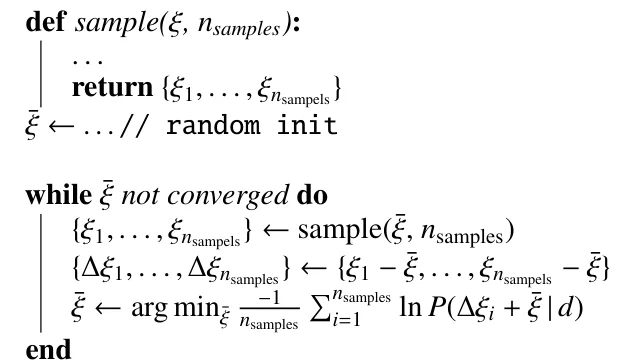
Pseudocode for our expansion point variational inference scheme using MGVI. }
11. Extinction Catalog
We release a catalog of expected extinction for all stars within the subset of the ZGR23 catalog that we use for our reconstruction (see \Cref{sec:data}). We predict the expected extinction conditional on the known parallax including parallax uncertainties. Our prediction is the best guess of our model for the extinction towards a star but is not necessarily the best guess for the extinction at the mean parallax of the star.
Our extinction predictions (see \Cref{sec:priors,sec:likelihood:response}) differ from the extinctions in the ZGR23 catalog by coupling the individual stars via the 3D dust extinction density. By virtue of every star depending on all nearby stars via the prior, our extinction predictions come in the form of joint predictions for all stars. In regions where the 3D dust extinction density is well constraint, the joint predictions to first order factorize into predictions for individual stars, and we can compute expected extinctions for individual stars and their uncertainties.
Our catalog of extinction includes the innermost 69pc from the beginning of our grid and the outer 550pc beyond 1.25kpc that we cut away in the 3D map. We advise caution when analyzing the stars of our catalog within those regions as they might carry additional biases. See \Cref{sec:caveats,sec:posterior_inference} for details on why these regions where removed from the final map.
Our extinction prediction versus the ZGR23 extinction.
 }}
}
}}
}
Our inferred uncertainties versus the ZGR23 extinction uncertainties.
 }}
}
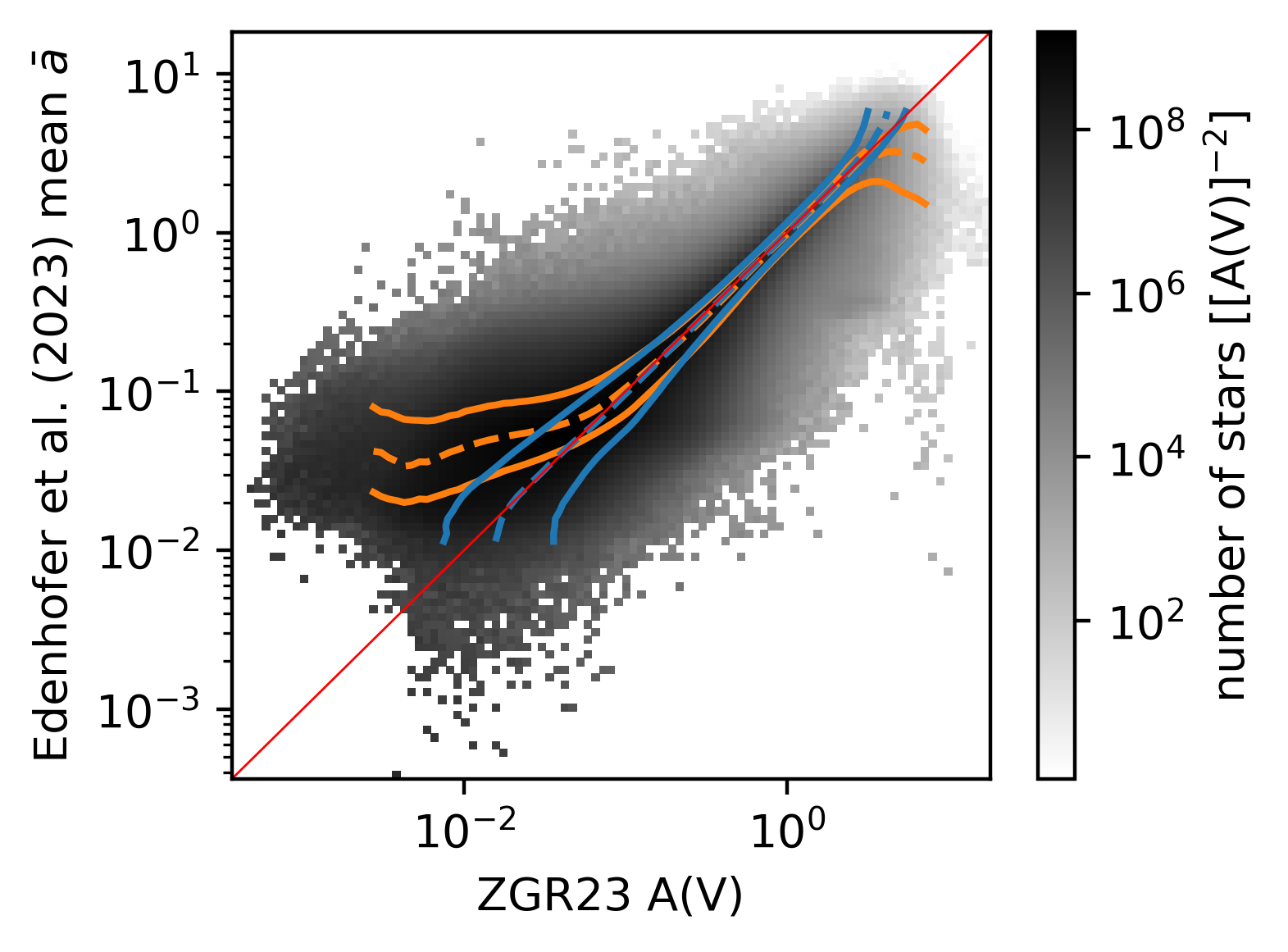
\caption{\label{fig:zgr23_versus_ours}%
The top panel shows our mean posterior extinctions versus the ZGR23 extinctions to stars as 2D histogram.
The $16^\text{th}$, $50^\text{th}$, and $84^\text{th}$ quantiles of the ZGR23 extinctions for each bin of our mean extinction are shown as blue lines.
The respective quantiles of our predictions in bins of the ZGR23 extinctions are shown as orange lines.
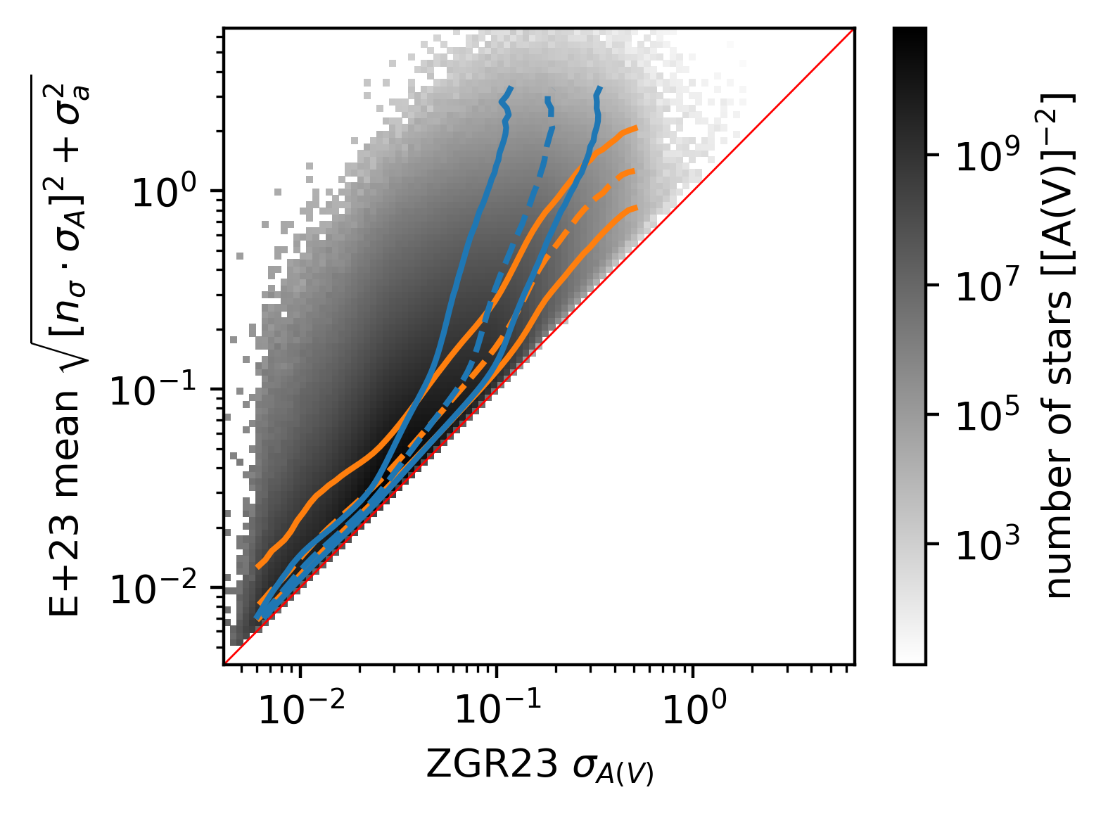
The bottom panel shows the same comparison but for our posterior mean predictions for the ZGR23 measurement uncertainties $\sqrt{\left[n_\sigma(\xi) \cdot \sigma_A\right]^2+\sigma_a^2}$ versus the ZGR23 uncertainties.
Note, the predictions for the ZGR23 measurement uncertainties are not the uncertainties of our extinction predictions.
See \Cref{sec:likelihood} and in specific \Cref{eq:total_likelihood} for further details on the quantities shown here.
The bisectors are shown in red.
The colorbars are logarithmic.
}
}}
}
\caption{\label{fig:zgr23_versus_ours}%
The top panel shows our mean posterior extinctions versus the ZGR23 extinctions to stars as 2D histogram.
The $16^\text{th}$, $50^\text{th}$, and $84^\text{th}$ quantiles of the ZGR23 extinctions for each bin of our mean extinction are shown as blue lines.
The respective quantiles of our predictions in bins of the ZGR23 extinctions are shown as orange lines.
The bottom panel shows the same comparison but for our posterior mean predictions for the ZGR23 measurement uncertainties $\sqrt{\left[n_\sigma(\xi) \cdot \sigma_A\right]^2+\sigma_a^2}$ versus the ZGR23 uncertainties.
Note, the predictions for the ZGR23 measurement uncertainties are not the uncertainties of our extinction predictions.
See \Cref{sec:likelihood} and in specific \Cref{eq:total_likelihood} for further details on the quantities shown here.
The bisectors are shown in red.
The colorbars are logarithmic.
}
The top panel of \Cref{fig:zgr23_versus_ours} compares the ZGR23 extinctions to our mean extinction predictions to stars. Overall, our mean extinctions are in very good agreement with the extinctions in the ZGR23 catalog for the vast majority of stars. However, below 50 mmag and above 4 mag our extinction predictions deviate from the predictions in ZGR23. At any given ZGR23 (respectively our) extinction bin, we would expect half of our (respectively the ZGR23) extinctions to be below and the other half to be above the bisector. At 50 mmag, 34% more stars than expected have higher extinctions than the corresponding extinctions in ZGR23. The difference further widens for lower ZGR23 extinctions. At 4 mag, 34% more stars than expected have lower extinctions than the corresponding extinctions in ZGR23.
The bottom panel of \Cref{fig:zgr23_versus_ours} shows our and the ZGR23 extinction uncertainties. Note, our extinction uncertainties are predictions for the measured uncertainties of the ZGR23 catalog $\left[n_\sigma(\xi) \cdot \sigma_A\right]^2+\sigma_a^2(\rho(\xi))$ and not the uncertainties of our extinction predictions $\mathrm{std}(\bar{a})$, see \Cref{sec:likelihood}. Overall, both uncertainties agree well for the vast majority of stars. At low extinctions uncertainties our uncertainties only marginally inflate the ZGR23 uncertainties. However, at high extinction uncertainties, our predictions cover a larger range, and we find that the ZGR23 significantly underpredicts our extinction uncertainties of stars.
 }}
\caption{%
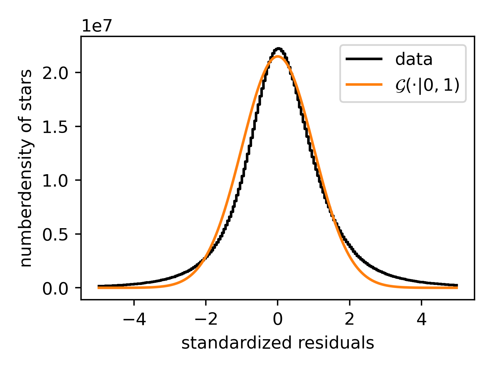
The mean standardized extinctions $(A - \bar{a}) / \sqrt{(n_\sigma \cdot \sigma_A)^2 + \sigma^2_a}$ (see \Cref{sec:likelihood} and in specific \Cref{eq:total_likelihood}) within the range of $-5$ to $5$.
}
}}
\caption{%
The mean standardized extinctions $(A - \bar{a}) / \sqrt{(n_\sigma \cdot \sigma_A)^2 + \sigma^2_a}$ (see \Cref{sec:likelihood} and in specific \Cref{eq:total_likelihood}) within the range of $-5$ to $5$.
}
\Cref{fig:standardized_extinction_prediction} summarizes the extinctions and the extinction uncertainties of both ZGR23 and our predictions into a single histogram of the mean standardized extinction. The mean standardized residuals follow a standard Gaussian (c.f. \Cref{sec:likelihood}). However, the mean standardized residuals have two slight overdensities at each tail of the Gaussian indicating some outliers are not yet fully captured by our inference of the uncertainties.
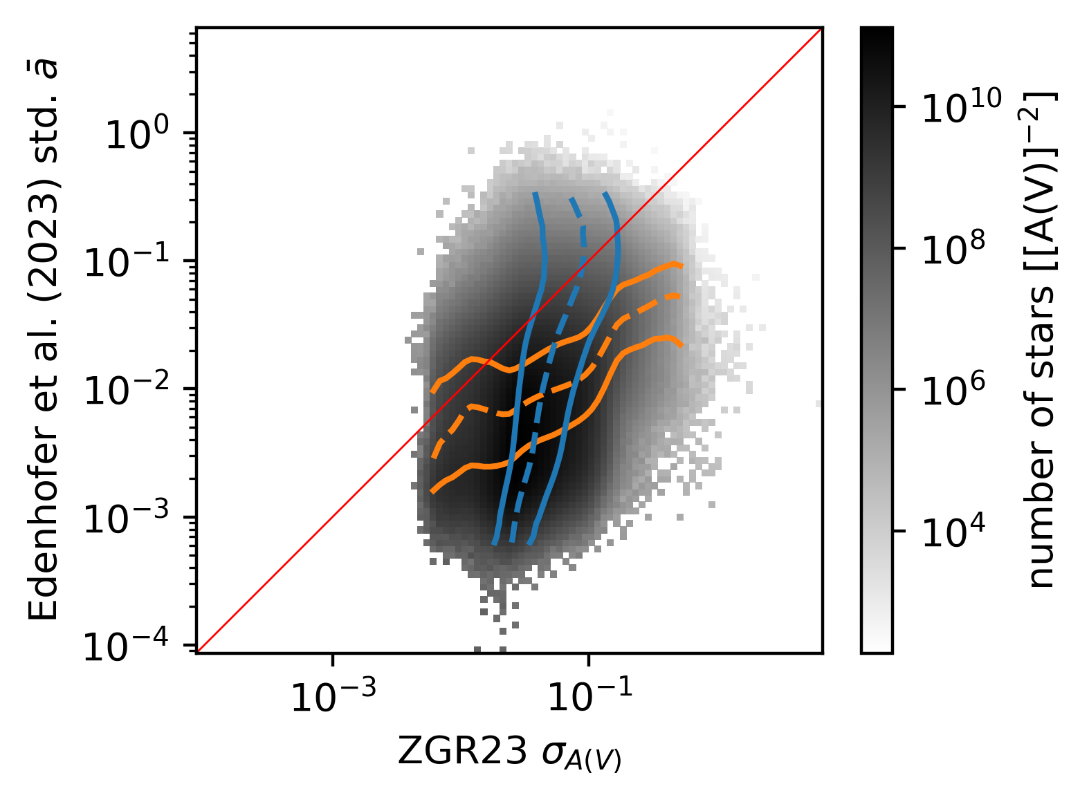 }}
\caption{\label{fig:actual_zgr23_versus_ours_unc}%
Similar to \Cref{fig:zgr23_versus_ours} but for the posterior standard deviation of our extinctions versus the ZGR23 uncertainties.
The $16^\text{th}$, $50^\text{th}$, and $84^\text{th}$ quantiles of the ZGR23 uncertainties for each bin of our standard deviation are shown as blue lines.
The respective quantiles of our standard deviation in bins of the ZGR23 uncertainties are shown as orange lines.
The bisectors are shown in red.
The colorbars are logarithmic.
}
}}
\caption{\label{fig:actual_zgr23_versus_ours_unc}%
Similar to \Cref{fig:zgr23_versus_ours} but for the posterior standard deviation of our extinctions versus the ZGR23 uncertainties.
The $16^\text{th}$, $50^\text{th}$, and $84^\text{th}$ quantiles of the ZGR23 uncertainties for each bin of our standard deviation are shown as blue lines.
The respective quantiles of our standard deviation in bins of the ZGR23 uncertainties are shown as orange lines.
The bisectors are shown in red.
The colorbars are logarithmic.
}
\Cref{fig:actual_zgr23_versus_ours_unc} shows the posterior standard deviation of our extinction predictions versus the ZGR23 uncertainties. Our model yields approximately one order in magnitude lower extinction uncertainties than the ZGR23 uncertainties for the vast majority of stars. The effect is less pronounced for low ZGR23 extinction uncertainties.
Our predictions for the extinction to stars theoretically contain more information since we allow for the cross-talk of nearby stars via the 3D distribution of dust and thus might be more accurate. However, the ZGR23 catalog might yield better results in practice because it does not discretize the 3D volume within which the stars reside. By discretizing the modeled volume we can produce contradicting data that in a continuous space is non-contradicting, e.g. by putting highly extincted stars that lie in a dust cloud into the same voxel as less extincted stars that are adjacent to the dust cloud. Overall, both predictions agree very well for stars below between 50 mmag and 4 mag. More work is needed to validate the discrepant predictions at very low and very high extinctions.
12. 2kpc Reconstruction
In \Cref{sec:posterior_inference} we describe how we iteratively increase the distance out to our maximum reconstructed distance.
We do so to improve the convergence of the reconstruction.
We also try naively reconstructing the full volume at once.
Using all the available data is computationally prohibitive, so we limit the reconstruction to high quality data using quality_flags==0, $\sigma_A \leq 0.04$, and ${\sigma_\omega}/{\omega} < 0.33$.
We use ${1}/{(\omega-\sigma_\omega)}<3\,\hbox{kpc}$ and ${1}/{(\omega+\sigma_\omega)}>40\,\hbox{pc}$ to select the stars within a 3kpc sphere. To further speed up the inference we start the inference using at first only a sample of $10%$, then $20%$, $45%$, $67%$ and finally $100%$ of the stars. In total, we select $59,334,214$ stars. After the inference, we cut away the outermost 1kpc of the sphere of the data constrained region to avoid degradation effects due to the thinning out of stars at the edge. The overall reconstructed volume after removing the outermost HEALPix spheres extends out to 2kpc in distance.
 }}
\caption{%
Axis parallel projections of the reconstructed dust extinction in a box of dimensions $4kpc \times 4kpc \times 0.8\,\hbox{kpc}$ centered on the Sun.
The colorbar is linear and saturates at the $99.9%$ quantile.
}
}}
\caption{%
Axis parallel projections of the reconstructed dust extinction in a box of dimensions $4kpc \times 4kpc \times 0.8\,\hbox{kpc}$ centered on the Sun.
The colorbar is linear and saturates at the $99.9%$ quantile.
}
 }}
\caption{%
Same as \Cref{fig:galactic_2kpc} but with a catalog of clusters of young stellar objects (Kuhn2023YSO) based on Kuhn2021, Winston2020, Marton2022 shown a blue dots on top of the reconstruction and their distance uncertainties shown as extended lines.
}
}}
\caption{%
Same as \Cref{fig:galactic_2kpc} but with a catalog of clusters of young stellar objects (Kuhn2023YSO) based on Kuhn2021, Winston2020, Marton2022 shown a blue dots on top of the reconstruction and their distance uncertainties shown as extended lines.
}
The reconstruction is shown in \Cref{fig:galactic_2kpc} and again in \Cref{fig:galactic_2kpc_with_ysos} with a catalog of YSO clusters (Kuhn2023YSO) overlaid on top. It shows the same large scale features as the smaller reconstruction discussed in the main text. The distribution of dense dust clouds is in agreement with the positions of YSO clusters within the distance uncertainties of the YSO clusters. Compared to \Cref{fig:galactic} the reconstruction is less detailed and features more pronounced artifacts.
We use the larger reconstruction to validate the inference of the smaller one. Specifically, we use the larger reconstruction to ensure that structures aligned with or close to the radial boundaries at which we increase the distance of the main reconstruction are independent of the locations at which we increase the distance covered.
We release the larger reconstruction as an additional data product together with the main reconstruction. We advise using the main reconstruction for all regions that fall within its volume. Care should be taken when interpreting small scale features or structures at high distances in the larger reconstruction.
13. Using the Reconstruction
All data products are made publicly available at https://doi.org/10.5281/zenodo.8187943. The data products are stored in the FITS file format. The main data products are the posterior samples of the spatial 3D distribution of dust extinction discretized to HEALPix spheres at logarithmically spaced distances. For convenience, we also provide the posterior mean and standard deviation of the samples of the HEALPix spheres at logarithmically spaced distances.
We additionally interpolate the posterior mean and standard deviation to a Cartesian grid. The interpolation is carried out at a lower resolution using $2^3\,\hbox{pc}^3$ voxels to keep the filesize reasonably small. We recommend re-interpolating the map at a higher resolution for the study of individual regions within the map.
We release the interpolation script as part of the data release.
Its signature reads interp2box.py [-h] [-o OUTPUT_DIRECTORY] [-b BOX] healpix_path.
A box is a string of two tuples separated by two colons.
The first tuple specifies the number of voxels along each axis of the box and the second tuple specifies the corners of the box in parsecs in heliocentric coordinates.
To interpolate the map to a box with $1051 \times 1051 \times 351$ voxels of size $\rm |X|, |Y| \leq 2100\,\hbox{pc}$ and $\rm |Z| \leq 700\,\hbox{pc}$, use
interp2box.py -b '(1051,1051,351)::((-2100,2100),(-2100,2100),(-700,700))' -- mean_and_std_healpix.fits.
In addition, we interpolate the posterior mean and standard deviation to galactic longitude, latitude and distance.
The signature of the interpolation script reads interp2lbd.py [-h] [-o OUTPUT_DIRECTORY] [-b BOX] healpix_path.
Its behavior is similar to interp2box.py but the box is specified in terms of galactic longitude, latitude and distance in units of degrees, degrees, and parsecs respectively.
Both scripts require the Python packages numpy (Harris2020), astropy (Astropy2013, Astropy2018, Astropy2022), and healpy (Gorski2005, Zonca2019).
Depending on the number of output voxels, the interpolation can be very memory intensive and computationally expensive.
Literature
- [Alves2020] Alves, João and Zucker, Catherine and Goodman, Alyssa A. and Speagle, Joshua S. and Meingast, Stefan and Robitaille, Thomas and Finkbeiner, Douglas P. and Schlafly, Edward F. and Green, Gregory M.: A Galactic-scale gas wave in the solar neighbourhood, Feb-2020, Nature, Vol. 578, Nr. 7794, pp. 237-239, https://doi.org/10.1038/s41586-019-1874-z
- [Anders2019] Anders, F. and Khalatyan, A. and Chiappini, C. and Queiroz, A.B. and Santiago, B.X. and Jordi, C. and Girardi, L. and Brown, A.G.A. and Matijevič, G. and Monari, G. and Cantat-Gaudin, T. and Weiler, M. and Khan, S. and Miglio, A. and Carrillo, I. and Romero-Gómez, M. and Minchev, I. and de Jong, R.S. and Antoja, T. and Ramos, P. and Steinmetz, M. and Enke, H.: Photo-astrometric distances, extinctions, and astrophysical parameters for Gaia DR2 stars brighter than G = 18, Aug-2019, Astronomy & Astrophysics, Vol. 628, pp. A94, https://doi.org/10.1051/0004-6361/201935765
- [Anders2022] Anders, F. and Khalatyan, A. and Queiroz, A.B.A. and Chiappini, C. and Ardèvol, J. and Casamiquela, L. and Figueras, F. and Jiménez-Arranz, Ó. and Jordi, C. and Monguió, M. and Romero-Gómez, M. and Altamirano, D. and Antoja, T. and Assaad, R. and Cantat-Gaudin, T. and Castro-Ginard, A. and Enke, H. and Girardi, L. and Guiglion, G. and Khan, S. and Luri, X. and Miglio, A. and Minchev, I. and Ramos, P. and Santiago, B.X. and Steinmetz, M.: Photo-astrometric distances, extinctions, and astrophysical parameters for Gaia EDR3 stars brighter than G = 18.5, Feb-2022, Astronomy & Astrophysics, Vol. 658, pp. A91, https://doi.org/10.1051/0004-6361/202142369
- [Arras2019] Arras, Philipp and Baltac, Mihai and Ensslin, Torsten A. and Frank, Philipp and Hutschenreuter, Sebastian and Knollmueller, Jakob and Leike, Reimar and Newrzella, Max-Niklas and Platz, Lukas and Reinecke, Martin and Stadler, Julia: NIFTy5: Numerical Information Field Theory v5, 03-2019
- [Arras2022] Arras, Philipp and Frank, Philipp and Haim, Philipp and Knollmüller, Jakob and Leike, Reimar and Reinecke, Martin and Enßlin, Torsten: Variable structures in M87* from space, time and frequency resolved interferometry, Jan-2022, Nature Astronomy, Vol. 6, pp. 259-269, https://doi.org/10.1038/s41550-021-01548-0
- [Astropy2013] Astropy Collaboration and Robitaille, Thomas P. and Tollerud, Erik J. and Greenfield, Perry and Droettboom, Michael and Bray, Erik and Aldcroft, Tom and Davis, Matt and Ginsburg, Adam and Price-Whelan, Adrian M. and Kerzendorf, Wolfgang E. and Conley, Alexander and Crighton, Neil and Barbary, Kyle and Muna, Demitri and Ferguson, Henry and Grollier, Frédéric and Parikh, Madhura M. and Nair, Prasanth H. and Unther, Hans M. and Deil, Christoph and Woillez, Julien and Conseil, Simon and Kramer, Roban and Turner, James E.H. and Singer, Leo and Fox, Ryan and Weaver, Benjamin A. and Zabalza, Victor and Edwards, Zachary I. and Azalee Bostroem, K. and Burke, D.J. and Casey, Andrew R. and Crawford, Steven M. and Dencheva, Nadia and Ely, Justin and Jenness, Tim and Labrie, Kathleen and Lim, Pey Lian and Pierfederici, Francesco and Pontzen, Andrew and Ptak, Andy and Refsdal, Brian and Servillat, Mathieu and Streicher, Ole: Astropy: A community Python package for astronomy, Oct-2013, Astronomy & Astrophysics, Vol. 558, pp. A33, https://doi.org/10.1051/0004-6361/201322068
- [Astropy2018] Astropy Collaboration and Price-Whelan, A.M. and Sipőcz, B.M. and Günther, H.M. and Lim, P.L. and Crawford, S.M. and Conseil, S. and Shupe, D.L. and Craig, M.W. and Dencheva, N. and Ginsburg, A. and VanderPlas, J.T. and Bradley, L.D. and Pérez-Suárez, D. and de Val-Borro, M. and Aldcroft, T.L. and Cruz, K.L. and Robitaille, T.P. and Tollerud, E.J. and Ardelean, C. and Babej, T. and Bach, Y.P. and Bachetti, M. and Bakanov, A.V. and Bamford, S.P. and Barentsen, G. and Barmby, P. and Baumbach, A. and Berry, K.L. and Biscani, F. and Boquien, M. and Bostroem, K.A. and Bouma, L.G. and Brammer, G.B. and Bray, E.M. and Breytenbach, H. and Buddelmeijer, H. and Burke, D.J. and Calderone, G. and Cano Rodr'\iguez, J.L. and Cara, M. and Cardoso, J.V.M. and Cheedella, S. and Copin, Y. and Corrales, L. and Crichton, D. and D'Avella, D. and Deil, C. and Depagne, É. and Dietrich, J.P. and Donath, A. and Droettboom, M. and Earl, N. and Erben, T. and Fabbro, S. and Ferreira, L.A. and Finethy, T. and Fox, R.T. and Garrison, L.H. and Gibbons, S.L.J. and Goldstein, D.A. and Gommers, R. and Greco, J.P. and Greenfield, P. and Groener, A.M. and Grollier, F. and Hagen, A. and Hirst, P. and Homeier, D. and Horton, A.J. and Hosseinzadeh, G. and Hu, L. and Hunkeler, J.S. and Ivezi'c, Ž. and Jain, A. and Jenness, T. and Kanarek, G. and Kendrew, S. and Kern, N.S. and Kerzendorf, W.E. and Khvalko, A. and King, J. and Kirkby, D. and Kulkarni, A.M. and Kumar, A. and Lee, A. and Lenz, D. and Littlefair, S.P. and Ma, Z. and Macleod, D.M. and Mastropietro, M. and McCully, C. and Montagnac, S. and Morris, B.M. and Mueller, M. and Mumford, S.J. and Muna, D. and Murphy, N.A. and Nelson, S. and Nguyen, G.H. and Ninan, J.P. and Nöthe, M. and Ogaz, S. and Oh, S. and Parejko, J.K. and Parley, N. and Pascual, S. and Patil, R. and Patil, A.A. and Plunkett, A.L. and Prochaska, J.X. and Rastogi, T. and Reddy Janga, V. and Sabater, J. and Sakurikar, P. and Seifert, M. and Sherbert, L.E. and Sherwood-Taylor, H. and Shih, A.Y. and Sick, J. and Silbiger, M.T. and Singanamalla, S. and Singer, L.P. and Sladen, P.H. and Sooley, K.A. and Sornarajah, S. and Streicher, O. and Teuben, P. and Thomas, S.W. and Tremblay, G.R. and Turner, J.E.H. and Terrón, V. and van Kerkwijk, M.H. and de la Vega, A. and Watkins, L.L. and Weaver, B.A. and Whitmore, J.B. and Woillez, J. and Zabalza, V. and Astropy Contributors: The Astropy Project: Building an Open-science Project and Status of the v2.0 Core Package, Sep-2018, Astronomical Journal, Vol. 156, Nr. 3, pp. 123, https://doi.org/10.3847/1538-3881/aabc4f
- [Astropy2022] Astropy Collaboration and Price-Whelan, Adrian M. and Lim, Pey Lian and Earl, Nicholas and Starkman, Nathaniel and Bradley, Larry and Shupe, David L. and Patil, Aarya A. and Corrales, Lia and Brasseur, C.E. and Nöthe, Maximilian and Donath, Axel and Tollerud, Erik and Morris, Brett M. and Ginsburg, Adam and Vaher, Eero and Weaver, Benjamin A. and Tocknell, James and Jamieson, William and van Kerkwijk, Marten H. and Robitaille, Thomas P. and Merry, Bruce and Bachetti, Matteo and Günther, H. Moritz and Aldcroft, Thomas L. and Alvarado-Montes, Jaime A. and Archibald, Anne M. and Bódi, Attila and Bapat, Shreyas and Barentsen, Geert and Bazán, Juanjo and Biswas, Manish and Boquien, Médéric and Burke, D.J. and Cara, Daria and Cara, Mihai and Conroy, Kyle E. and Conseil, Simon and Craig, Matthew W. and Cross, Robert M. and Cruz, Kelle L. and D'Eugenio, Francesco and Dencheva, Nadia and Devillepoix, Hadrien A.R. and Dietrich, Jörg P. and Eigenbrot, Arthur Davis and Erben, Thomas and Ferreira, Leonardo and Foreman-Mackey, Daniel and Fox, Ryan and Freij, Nabil and Garg, Suyog and Geda, Robel and Glattly, Lauren and Gondhalekar, Yash and Gordon, Karl D. and Grant, David and Greenfield, Perry and Groener, Austen M. and Guest, Steve and Gurovich, Sebastian and Handberg, Rasmus and Hart, Akeem and Hatfield-Dodds, Zac and Homeier, Derek and Hosseinzadeh, Griffin and Jenness, Tim and Jones, Craig K. and Joseph, Prajwel and Kalmbach, J. Bryce and Karamehmetoglu, Emir and Ka\luszy'nski, Miko\laj and Kelley, Michael S.P. and Kern, Nicholas and Kerzendorf, Wolfgang E. and Koch, Eric W. and Kulumani, Shankar and Lee, Antony and Ly, Chun and Ma, Zhiyuan and MacBride, Conor and Maljaars, Jakob M. and Muna, Demitri and Murphy, N.A. and Norman, Henrik and O'Steen, Richard and Oman, Kyle A. and Pacifici, Camilla and Pascual, Sergio and Pascual-Granado, J. and Patil, Rohit R. and Perren, Gabriel I. and Pickering, Timothy E. and Rastogi, Tanuj and Roulston, Benjamin R. and Ryan, Daniel F. and Rykoff, Eli S. and Sabater, Jose and Sakurikar, Parikshit and Salgado, Jesús and Sanghi, Aniket and Saunders, Nicholas and Savchenko, Volodymyr and Schwardt, Ludwig and Seifert-Eckert, Michael and Shih, Albert Y. and Jain, Anany Shrey and Shukla, Gyanendra and Sick, Jonathan and Simpson, Chris and Singanamalla, Sudheesh and Singer, Leo P. and Singhal, Jaladh and Sinha, Manodeep and Sipőcz, Brigitta M. and Spitler, Lee R. and Stansby, David and Streicher, Ole and Šumak, Jani and Swinbank, John D. and Taranu, Dan S. and Tewary, Nikita and Tremblay, Grant R. and de Val-Borro, Miguel and Van Kooten, Samuel J. and Vasovi'c, Zlatan and Verma, Shresth and de Miranda Cardoso, José Vin'\icius and Williams, Peter K.G. and Wilson, Tom J. and Winkel, Benjamin and Wood-Vasey, W.M. and Xue, Rui and Yoachim, Peter and Zhang, Chen and Zonca, Andrea and Astropy Project Contributors: The Astropy Project: Sustaining and Growing a Community-oriented Open-source Project and the Latest Major Release (v5.0) of the Core Package, Aug-2022, The Astrophysical Journal, Vol. 935, Nr. 2, pp. 167, https://doi.org/10.3847/1538-4357/ac7c74
- [CantatGaudin2022] Tristan Cantat-Gaudin and Morgan Fouesneau and Hans-Walter Rix and Anthony G. A. Brown and Alfred Castro-Ginard and Zuzanna Kostrzewa-Rutkowska and Ronald Drimmel and David W. Hogg and Andrew R. Casey and Shourya Khanna and Semyeong Oh and Adrian M. Price-Whelan and Vasily Belokurov and Andrew K. Saydjari and G. Green: An empirical model of the $\less$i$\greater$Gaia$\less$/i$\greater$ DR3 selection function, Jan-2023, Astronomy & Astrophysics, Vol. 669, pp. A55, https://doi.org/10.1051/0004-6361/202244784
- [Capitanio2017] Capitanio, L. and Lallement, R. and Vergely, J.L. and Elyajouri, M. and Monreal-Ibero, A.: Three-dimensional mapping of the local interstellar medium with composite data, Oct-2017, Astronomy & Astrophysics, Vol. 606, pp. A65, https://doi.org/10.1051/0004-6361/201730831
- [Carasco2021] Carrasco, J.M. and Weiler, M. and Jordi, C. and Fabricius, C. and De Angeli, F. and Evans, D.W. and van Leeuwen, F. and Riello, M. and Montegriffo, P.: Internal calibration of Gaia BP/RP low-resolution spectra, Aug-2021, Astronomy & Astrophysics, Vol. 652, pp. A86, https://doi.org/10.1051/0004-6361/202141249
- [chambers2019] K. C. Chambers and E. A. Magnier and N. Metcalfe and H. A. Flewelling and M. E. Huber and C. Z. Waters and L. Denneau and P. W. Draper and D. Farrow and D. P. Finkbeiner and C. Holmberg and J. Koppenhoefer and P. A. Price and A. Rest and R. P. Saglia and E. F. Schlafly and S. J. Smartt and W. Sweeney and R. J. Wainscoat and W. S. Burgett and S. Chastel and T. Grav and J. N. Heasley and K. W. Hodapp and R. Jedicke and N. Kaiser and R. -P. Kudritzki and G. A. Luppino and R. H. Lupton and D. G. Monet and J. S. Morgan and P. M. Onaka and B. Shiao and C. W. Stubbs and J. L. Tonry and R. White and E. Bañados and E. F. Bell and R. Bender and E. J. Bernard and M. Boegner and F. Boffi and M. T. Botticella and A. Calamida and S. Casertano and W. -P. Chen and X. Chen and S. Cole and N. Deacon and C. Frenk and A. Fitzsimmons and S. Gezari and V. Gibbs and C. Goessl and T. Goggia and R. Gourgue and B. Goldman and P. Grant and E. K. Grebel and N. C. Hambly and G. Hasinger and A. F. Heavens and T. M. Heckman and R. Henderson and T. Henning and M. Holman and U. Hopp and W. -H. Ip and S. Isani and M. Jackson and C. D. Keyes and A. M. Koekemoer and R. Kotak and D. Le and D. Liska and K. S. Long and J. R. Lucey and M. Liu and N. F. Martin and G. Masci and B. McLean and E. Mindel and P. Misra and E. Morganson and D. N. A. Murphy and A. Obaika and G. Narayan and M. A. Nieto-Santisteban and P. Norberg and J. A. Peacock and E. A. Pier and M. Postman and N. Primak and C. Rae and A. Rai and A. Riess and A. Riffeser and H. W. Rix and S. Röser and R. Russel and L. Rutz and E. Schilbach and A. S. B. Schultz and D. Scolnic and L. Strolger and A. Szalay and S. Seitz and E. Small and K. W. Smith and D. R. Soderblom and P. Taylor and R. Thomson and A. N. Taylor and A. R. Thakar and J. Thiel and D. Thilker and D. Unger and Y. Urata and J. Valenti and J. Wagner and T. Walder and F. Walter and S. P. Watters and S. Werner and W. M. Wood-Vasey and R. Wyse: The Pan-STARRS1 Surveys, 2019
- [Chen2018] Li, Linlin and Shen, Shiyin and Hou, Jinliang and Yuan, Haibo and Xiang, Maosheng and Chen, Bingqiu and Huang, Yang and Liu, Xiaowei: Three-dimensional Structure of the Milky Way Dust: Modeling of LAMOST Data, May-2018, The Astrophysical Journal, Vol. 858, Nr. 2, pp. 75, https://doi.org/10.3847/1538-4357/aabaef
- [Chen2019] Chen, B. -Q. and Huang, Y. and Yuan, H. -B. and Wang, C. and Fan, D. -W. and Xiang, M. -S. and Zhang, H. -W. and Tian, Z. -J. and Liu, X. -W.: Three-dimensional interstellar dust reddening maps of the Galactic plane, Mar-2019, Monthly Notices of the RAS, Vol. 483, Nr. 4, pp. 4277-4289, https://doi.org/10.1093/mnras/sty3341
- [DeAngeli2022] De Angeli, F. and Weiler, M. and Montegriffo, P. and Evans, D.W. and Riello, M. and Andrae, R. and Carrasco, J.M. and Busso, G. and Burgess, P.W. and Cacciari, C. and Davidson, M. and Harrison, D.L. and Hodgkin, S.T. and Jordi, C. and Osborne, P.J. and Pancino, E. and Altavilla, G. and Barstow, M.A. and Bailer-Jones, C.A.L. and Bellazzini, M. and Brown, A.G.A. and Castellani, M. and Cowell, S. and Delchambre, L. and De Luise, F. and Diener, C. and Fabricius, C. and Fouesneau, M. and Fremat, Y. and Gilmore, G. and Giuffrida, G. and Hambly, N.C. and Hidalgo, S. and Holland, G. and Kostrzewa-Rutkowska, Z. and van Leeuwen, F. and Lobel, A. and Marinoni, S. and Miller, N. and Pagani, C. and Palaversa, L. and Piersimoni, A.M. and Pulone, L. and Ragaini, S. and Rainer, M. and Richards, P.J. and Rixon, G.T. and Ruz-Mieres, D. and Sanna, N. and Sarro, L.M. and Rowell, N. and Sordo, R. and Walton, N.A. and Yoldas, A.: Gaia Data Release 3: Processing and validation of BP/RP low-resolution spectral data, Jun-2022, arXiv e-prints, pp. arXiv:2206.06143, https://doi.org/10.48550/arXiv.2206.06143
- [Delchambre2022] Delchambre, L. and Bailer-Jones, C.A.L. and Bellas-Velidis, I. and Drimmel, R. and Garabato, D. and Carballo, R. and Hatzidimitriou, D. and Marshall, D.J. and Andrae, R. and Dafonte, C. and Livanou, E. and Fouesneau, M. and Licata, E.L. and Lindstrom, H.E.P. and Manteiga, M. and Robin, C. and Silvelo, A. and Abreu Aramburu, A. and Alvarez, M.A. and Bakker, J. and Bijaoui, A. and Brouillet, N. and Brugaletta, E. and Burlacu, A. and Casamiquela, L. and Chaoul, L. and Chiavassa, A. and Contursi, G. and Cooper, W.J. and Creevey, O.L. and Dapergolas, A. and de Laverny, P. and Demouchy, C. and Dharmawardena, T.E. and Edvardsson, B. and Fremat, Y. and Garcia-Lario, P. and Garcia-Torres, M. and Gavel, A. and Gomez, A. and Gonzalez-Santamaria, I. and Heiter, U. and Jean-Antoine Piccolo, A. and Kontizas, M. and Kordopatis, G. and Korn, A.J. and Lanzafame, A.C. and Lebreton, Y. and Lobel, A. and Lorca, A. and Magdaleno Romeo, A. and Marocco, F. and Mary, N. and Nicolas, C. and Ordenovic, C. and Pailler, F. and Palicio, P.A. and Pallas-Quintela, L. and Panem, C. and Pichon, B. and Poggio, E. and Recio-Blanco, A. and Riclet, F. and Rybizki, J. and Santovena, R. and Sarro, L.M. and Schultheis, M.S. and Segol, M. and Slezak, I. and Smart, R.L. and Sordo, R. and Soubiran, C. and Suveges, M. and Thevenin, F. and Torralba Elipe, G. and Ulla, A. and Utrilla, E. and Vallenari, A. and van Dillen, E. and Zhao, H. and Zorec, J.: Gaia DR3: Apsis III -- Non-stellar content and source classification, Jun-2022, arXiv e-prints, pp. arXiv:2206.06710, https://doi.org/10.48550/arXiv.2206.06710
- [Dharmawardena2022] Dharmawardena, T.E. and Bailer-Jones, C.A.L. and Fouesneau, M. and Foreman-Mackey, D.: Three-dimensional dust density structure of the Orion, Cygnus X, Taurus, and Perseus star-forming regions, Feb-2022, Astronomy & Astrophysics, Vol. 658, pp. A166, https://doi.org/10.1051/0004-6361/202141298
- [Draine2011] Draine, Bruce T.: Physics of the Interstellar and Intergalactic Medium, 2011
- [Edenhofer2022] Edenhofer, Gordian and Leike, Reimar H. and Frank, Philipp and Enßlin, Torsten A.: Sparse Kernel Gaussian Processes through Iterative Charted Refinement (ICR), 2022, https://doi.org/10.48550/ARXIV.2206.10634
- [Edenhofer2023NIFTyRE] Edenhofer, Gordian and Frank, Philipp and Leike, Reimar H. and Roth, Jakob and Guerdi, Massin and Enßlin, Torsten A.: Re-Envisioning Numerical Information Field Theory (NIFTy): An Inference Library for Gaussian Processes and Variational Inference, 2023
- [Frank2021] Philipp Frank and Reimar Leike and Torsten A. Enßlin: Geometric Variational Inference, Jul-2021, Entropy, Vol. 23, Nr. 7, pp. 853, https://doi.org/10.3390/e23070853
- [Frank2022] Frank, Philipp: Geometric Variational Inference and Its Application to Bayesian Imaging, 2022, Physical Sciences Forum, Vol. 5, Nr. 1, https://doi.org/10.3390/psf2022005006
- [GaiaCollaboration2022] Gaia Collaboration and Vallenari, A. and Brown, A.G.A. and Prusti, T. and de Bruijne, J.H.J. and Arenou, F. and Babusiaux, C. and Biermann, M. and Creevey, O.L. and Ducourant, C. and Evans, D.W. and Eyer, L. and Guerra, R. and Hutton, A. and Jordi, C. and Klioner, S.A. and Lammers, U.L. and Lindegren, L. and Luri, X. and Mignard, F. and Panem, C. and Pourbaix, D. and Randich, S. and Sartoretti, P. and Soubiran, C. and Tanga, P. and Walton, N.A. and Bailer-Jones, C.A.L. and Bastian, U. and Drimmel, R. and Jansen, F. and Katz, D. and Lattanzi, M.G. and van Leeuwen, F. and Bakker, J. and Cacciari, C. and Castañeda, J. and De Angeli, F. and Fabricius, C. and Fouesneau, M. and Frémat, Y. and Galluccio, L. and Guerrier, A. and Heiter, U. and Masana, E. and Messineo, R. and Mowlavi, N. and Nicolas, C. and Nienartowicz, K. and Pailler, F. and Panuzzo, P. and Riclet, F. and Roux, W. and Seabroke, G.M. and Sordo\orcit, R. and Thévenin, F. and Gracia-Abril, G. and Portell, J. and Teyssier, D. and Altmann, M. and Andrae, R. and Audard, M. and Bellas-Velidis, I. and Benson, K. and Berthier, J. and Blomme, R. and Burgess, P.W. and Busonero, D. and Busso, G. and Cánovas, H. and Carry, B. and Cellino, A. and Cheek, N. and Clementini, G. and Damerdji, Y. and Davidson, M. and de Teodoro, P. and Nuñez Campos, M. and Delchambre, L. and Dell'Oro, A. and Esquej, P. and Fernández-Hernández, J. and Fraile, E. and Garabato, D. and Garc'\ia-Lario, P. and Gosset, E. and Haigron, R. and Halbwachs, J. -L. and Hambly, N.C. and Harrison, D.L. and Hernández, J. and Hestroffer, D. and Hodgkin, S.T. and Holl, B. and Janßen, K. and Jevardat de Fombelle, G. and Jordan, S. and Krone-Martins, A. and Lanzafame, A.C. and Löffler, W. and Marchal, O. and Marrese, P.M. and Moitinho, A. and Muinonen, K. and Osborne, P. and Pancino, E. and Pauwels, T. and Recio-Blanco, A. and Reylé, C. and Riello, M. and Rimoldini, L. and Roegiers, T. and Rybizki, J. and Sarro, L.M. and Siopis, C. and Smith, M. and Sozzetti, A. and Utrilla, E. and van Leeuwen, M. and Abbas, U. and Ábrahám, P. and Abreu Aramburu, A. and Aerts, C. and Aguado, J.J. and Ajaj, M. and Aldea-Montero, F. and Altavilla, G. and Álvarez, M.A. and Alves, J. and Anders, F. and Anderson, R.I. and Anglada Varela, E. and Antoja, T. and Baines, D. and Baker, S.G. and Balaguer-Núñez, L. and Balbinot, E. and Balog, Z. and Barache, C. and Barbato, D. and Barros, M. and Barstow, M.A. and Bartolomé, S. and Bassilana, J. -L. and Bauchet, N. and Becciani, U. and Bellazzini, M. and Berihuete, A. and Bernet, M. and Bertone, S. and Bianchi, L. and Binnenfeld, A. and Blanco-Cuaresma, S. and Blazere, A. and Boch, T. and Bombrun, A. and Bossini, D. and Bouquillon, S. and Bragaglia, A. and Bramante, L. and Breedt, E. and Bressan, A. and Brouillet, N. and Brugaletta, E. and Bucciarelli, B. and Burlacu, A. and Butkevich, A.G. and Buzzi, R. and Caffau, E. and Cancelliere, R. and Cantat-Gaudin, T. and Carballo, R. and Carlucci, T. and Carnerero, M.I. and Carrasco, J.M. and Casamiquela, L. and Castellani, M. and Castro-Ginard, A. and Chaoul, L. and Charlot, P. and Chemin, L. and Chiaramida, V. and Chiavassa, A. and Chornay, N. and Comoretto, G. and Contursi, G. and Cooper, W.J. and Cornez, T. and Cowell, S. and Crifo, F. and Cropper, M. and Crosta, M. and Crowley, C. and Dafonte, C. and Dapergolas, A. and David, M. and David, P. and de Laverny, P. and De Luise, F. and De March, R. and De Ridder, J. and de Souza, R. and de Torres, A. and del Peloso, E.F. and del Pozo, E. and Delbo, M. and Delgado, A. and Delisle, J. -B. and Demouchy, C. and Dharmawardena, T.E. and Di Matteo, P. and Diakite, S. and Diener, C. and Distefano, E. and Dolding, C. and Edvardsson, B. and Enke, H. and Fabre, C. and Fabrizio, M. and Faigler, S. and Fedorets, G. and Fernique, P. and Fienga, A. and Figueras, F. and Fournier, Y. and Fouron, C. and Fragkoudi, F. and Gai, M. and Garcia-Gutierrez, A. and Garcia-Reinaldos, M. and Garc'\ia-Torres, M. and Garofalo, A. and Gavel, A. and Gavras, P. and Gerlach, E. and Geyer, R. and Giacobbe, P. and Gilmore, G. and Girona, S. and Giuffrida, G. and Gomel, R. and Gomez, A. and González-Núñez, J. and González-Santamar'\ia, I. and González-Vidal, J.J. and Granvik, M. and Guillout, P. and Guiraud, J. and Gutiérrez-Sánchez, R. and Guy, L.P. and Hatzidimitriou, D. and Hauser, M. and Haywood, M. and Helmer, A. and Helmi, A. and Sarmiento, M.H. and Hidalgo, S.L. and Hilger, T. and H\ladczuk, N. and Hobbs, D. and Holland, G. and Huckle, H.E. and Jardine, K. and Jasniewicz, G. and Jean-Antoine Piccolo, A. and Jiménez-Arranz, Ó. and Jorissen, A. and Juaristi Campillo, J. and Julbe, F. and Karbevska, L. and Kervella, P. and Khanna, S. and Kontizas, M. and Kordopatis, G. and Korn, A.J. and Kóspál, Á and Kostrzewa-Rutkowska, Z. and Kruszy'nska, K. and Kun, M. and Laizeau, P. and Lambert, S. and Lanza, A.F. and Lasne, Y. and Le Campion, J. -F. and Lebreton, Y. and Lebzelter, T. and Leccia, S. and Leclerc, N. and Lecoeur-Taibi, I. and Liao, S. and Licata, E.L. and Lindstr\om, H.E.P. and Lister, T.A. and Livanou, E. and Lobel, A. and Lorca, A. and Loup, C. and Madrero Pardo, P. and Magdaleno Romeo, A. and Managau, S. and Mann, R.G. and Manteiga, M. and Marchant, J.M. and Marconi, M. and Marcos, J. and Marcos Santos, M.M.S. and Mar'\in Pina, D. and Marinoni, S. and Marocco, F. and Marshall, D.J. and Polo, L. Martin and Mart'\in-Fleitas, J.M. and Marton, G. and Mary, N. and Masip, A. and Massari, D. and Mastrobuono-Battisti, A. and Mazeh, T. and McMillan, P.J. and Messina, S. and Michalik, D. and Millar, N.R. and Mints, A. and Molina, D. and Molinaro, R. and Molnár, L. and Monari, G. and Monguió, M. and Montegriffo, P. and Montero, A. and Mor, R. and Mora, A. and Morbidelli, R. and Morel, T. and Morris, D. and Muraveva, T. and Murphy, C.P. and Musella, I. and Nagy, Z. and Noval, L. and Ocaña, F. and Ogden, A. and Ordenovic, C. and Osinde, J.O. and Pagani, C. and Pagano, I. and Palaversa, L. and Palicio, P.A. and Pallas-Quintela, L. and Panahi, A. and Payne-Wardenaar, S. and Peñalosa Esteller, X. and Penttilä, A. and Pichon, B. and Piersimoni, A.M. and Pineau, F. -X. and Plachy, E. and Plum, G. and Poggio, E. and Prša, A. and Pulone, L. and Racero, E. and Ragaini, S. and Rainer, M. and Raiteri, C.M. and Rambaux, N. and Ramos, P. and Ramos-Lerate, M. and Re Fiorentin, P. and Regibo, S. and Richards, P.J. and Rios Diaz, C. and Ripepi, V. and Riva, A. and Rix, H. -W. and Rixon, G. and Robichon, N. and Robin, A.C. and Robin, C. and Roelens, M. and Rogues, H.R.O. and Rohrbasser, L. and Romero-Gómez, M. and Rowell, N. and Royer, F. and Ruz Mieres, D. and Rybicki, K.A. and Sadowski, G. and Sáez Núñez, A. and Sagristà Sellés, A. and Sahlmann, J. and Salguero, E. and Samaras, N. and Sanchez Gimenez, V. and Sanna, N. and Santoveña, R. and Sarasso, M. and Schultheis, M. and Sciacca, E. and Segol, M. and Segovia, J.C. and Ségransan, D. and Semeux, D. and Shahaf, S. and Siddiqui, H.I. and Siebert, A. and Siltala, L. and Silvelo, A. and Slezak, E. and Slezak, I. and Smart, R.L. and Snaith, O.N. and Solano, E. and Solitro, F. and Souami, D. and Souchay, J. and Spagna, A. and Spina, L. and Spoto, F. and Steele, I.A. and Steidelmüller, H. and Stephenson, C.A. and Süveges, M. and Surdej, J. and Szabados, L. and Szegedi-Elek, E. and Taris, F. and Taylo, M.B. and Teixeira, R. and Tolomei, L. and Tonello, N. and Torra, F. and Torra, J. and Torralba Elipe, G. and Trabucchi, M. and Tsounis, A.T. and Turon, C. and Ulla, A. and Unger, N. and Vaillant, M.V. and van Dillen, E. and van Reeven, W. and Vanel, O. and Vecchiato, A. and Viala, Y. and Vicente, D. and Voutsinas, S. and Weiler, M. and Wevers, T. and Wyrzykowski, L. and Yoldas, A. and Yvard, P. and Zhao, H. and Zorec, J. and Zucker, S. and Zwitter, T.: Gaia Data Release 3: Summary of the content and survey properties, Jul-2022, arXiv e-prints, pp. arXiv:2208.00211, https://doi.org/10.48550/arXiv.2208.00211
- [Gorski2005] Górski, K.M. and Hivon, E. and Banday, A.J. and : HEALPix: A Framework for High-Resolution Discretization and Fast Analysis of Data Distributed on the Sphere, Apr-2005, The Astrophysical Journal, Vol. 622, pp. 759-771, https://doi.org/10.1086/427976
- [Green2017] Green, Gregory M. and Schlafly, Edward F. and Finkbeiner, Douglas and Rix, Hans-Walter and Martin, Nicolas and Burgett, William and Draper, Peter W. and Flewelling, Heather and Hodapp, Klaus and Kaiser, Nicholas and Kudritzki, Rolf-Peter and Magnier, Eugene A. and Metcalfe, Nigel and Tonry, John L. and Wainscoat, Richard and Waters, Christopher: Galactic reddening in 3D from stellar photometry - an improved map, Jul-2018, Monthly Notices of the RAS, Vol. 478, Nr. 1, pp. 651-666, https://doi.org/10.1093/mnras/sty1008
- [Green2018] Green, Gregory M.: dustmaps: A Python interface for maps of interstellar dust, Jun-2018, The Journal of Open Source Software, Vol. 3, Nr. 26, pp. 695, https://doi.org/10.21105/joss.00695
- [Green2018Dustmaps] Green, Gregory M.: dustmaps: A Python interface for maps of interstellar dust, Jun-2018, The Journal of Open Source Software, Vol. 3, Nr. 26, pp. 695, https://doi.org/10.21105/joss.00695
- [Green2019] Green, Gregory M. and Schlafly, Edward and Zucker, Catherine and Speagle, Joshua S. and Finkbeiner, Douglas: A 3D Dust Map Based on Gaia, Pan-STARRS 1, and 2MASS, Dec-2019, The Astrophysical Journal, Vol. 887, Nr. 1, pp. 93, https://doi.org/10.3847/1538-4357/ab5362
- [Harris2020] Charles R. Harris and K. Jarrod Millman and St'efan J.: Array programming with NumPy, Sep-2020, Nature, Vol. 585, Nr. 7825, pp. 357--362, https://doi.org/10.1038/s41586-020-2649-2
- [Hoffman2011] Hoffman, Matthew D. and Gelman, Andrew: The No-U-Turn Sampler: Adaptively Setting Path Lengths in Hamiltonian Monte Carlo, Jan-2014, J. Mach. Learn. Res., Vol. 15, Nr. 1, pp. 1593–1623
- [Hutschenreuter2022] Hutschenreuter, S. and Anderson, C.S. and Betti, S. and Bower, G.C. and Brown, J. -A. and Brüggen, M. and Carretti, E. and Clarke, T. and Clegg, A. and Costa, A. and Croft, S. and Van Eck, C. and Gaensler, B.M. and de Gasperin, F. and Haverkorn, M. and Heald, G. and Hull, C.L.H. and Inoue, M. and Johnston-Hollitt, M. and Kaczmarek, J. and Law, C. and Ma, Y.K. and MacMahon, D. and Mao, S.A. and Riseley, C. and Roy, S. and Shanahan, R. and Shimwell, T. and Stil, J. and Sobey, C. and O'Sullivan, S.P. and Tasse, C. and Vacca, V. and Vernstrom, T. and Williams, P.K.G. and Wright, M. and Enßlin, T.A.: The Galactic Faraday rotation sky 2020, Jan-2022, Astronomy & Astrophysics, Vol. 657, pp. A43, https://doi.org/10.1051/0004-6361/202140486
- [Hutschenreuter2023] Hutschenreuter, Sebastian and Haverkorn, Marijke and Frank, Philipp and Raycheva, Nergis C. and Enßlin, Torsten A.: Disentangling the Faraday rotation sky, Apr-2023, arXiv e-prints, pp. arXiv:2304.12350, https://doi.org/10.48550/arXiv.2304.12350
- [Jax2018] James Bradbury and Roy Frostig and Peter Hawkins and Matthew James Johnson and Chris Leary and Dougal Maclaurin and George Necula and Adam Paszke and Jake VanderPlas and Skye Wanderman-Milne and Qiao Zhang: JAX: composable transformations of Python+NumPy programs, 2018, http://github.com/google/jax
- [Knollmueller2019] Knollmüller, Jakob and Enßlin, Torsten A.: Metric Gaussian Variational Inference, 2019, https://doi.org/10.48550/ARXIV.1901.11033
- [Kuhn2021] Kuhn, Michael A. and de Souza, Rafael S. and Krone-Martins, Alberto and Castro-Ginard, Alfred and Ishida, Emille E.O. and Povich, Matthew S. and Hillenbrand, Lynne A. and COIN Collaboration: SPICY: The Spitzer/IRAC Candidate YSO Catalog for the Inner Galactic Midplane, Jun-2021, Astrophysical Journal, Supplement, Vol. 254, Nr. 2, pp. 33, https://doi.org/10.3847/1538-4365/abe465
- [Kuhn2023YSO] Kuhn, Mike: personal communication, 2023-05-1
- [Lallement2018] Lallement, R. and Capitanio, L. and Ruiz-Dern, L. and Danielski, C. and Babusiaux, C. and Vergely, L. and Elyajouri, M. and Arenou, F. and Leclerc, N.: Three-dimensional maps of interstellar dust in the Local Arm: using Gaia, 2MASS, and APOGEE-DR14, Aug-2018, Astronomy & Astrophysics, Vol. 616, pp. A132, https://doi.org/10.1051/0004-6361/201832832
- [Lallement2019] Lallement, R. and Babusiaux, C. and Vergely, J.L. and Katz, D. and Arenou, F. and Valette, B. and Hottier, C. and Capitanio, L.: Gaia-2MASS 3D maps of Galactic interstellar dust within 3 kpc, May-2019, Astronomy & Astrophysics, Vol. 625, pp. A135, https://doi.org/10.1051/0004-6361/201834695
- [Lallement2022] Lallement, R. and Vergely, J.L. and Babusiaux, C. and Cox, N.L.J.: Updated Gaia-2MASS 3D maps of Galactic interstellar dust, May-2022, Astronomy & Astrophysics, Vol. 661, pp. A147, https://doi.org/10.1051/0004-6361/202142846
- [Leike2019] Leike, RH and Enßlin, TA: Charting nearby dust clouds using Gaia data only, 2019, Astronomy & Astrophysics, Vol. 631, pp. A32
- [Leike2020] Leike,R.L. and Glatzle,M. and Enßlin,T.A.: Resolving nearby dust clouds, 2020, Astronomy & Astrophysics, Vol. 639, pp. A138
- [Leike2022] Leike, R.H. and Edenhofer, G. and Knollmüller, J. and Alig, C. and Frank, P. and Enßlin, T.A.: The Galactic 3D large-scale dust distribution via Gaussian process regression on spherical coordinates, Apr-2022, arXiv e-prints, pp. arXiv:2204.11715, https://doi.org/10.48550/arXiv.2204.11715
- [Marton2022] Marton, Gábor and Ábrahám, Péter and Rimoldini, Lorenzo and Audard, Marc and Kun, Mária and Nagy, Zsófia and Kóspál, Ágnes and Szabados, László and Holl, Berry and Gavras, Panagiotis and Mowlavi, Nami and Nienartowicz, Krzysztof and Jevardat de Fombelle, Grégory and Lecoeur-Taïbi, Isabelle and Karbevska, Lea and Garcia-Lario, Pedro and Eyer, Laurent: Gaia Data Release 3 Validating the classification of variable Young Stellar Object candidates, Jun-2022, arXiv e-prints, pp. arXiv:2206.05796, https://doi.org/10.48550/arXiv.2206.05796
- [Mertsch2023] Mertsch, P. and Phan, V.H.M.: Bayesian inference of three-dimensional gas maps. II. Galactic HI, Mar-2023, Astronomy & Astrophysics, Vol. 671, pp. A54, https://doi.org/10.1051/0004-6361/202243326
- [Montegriffo2022] Montegriffo, P. and De Angeli, F. and Andrae, R. and Riello, M. and Pancino, E. and Sanna, N. and Bellazzini, M. and Evans, D.W. and Carrasco, J.M. and Sordo, R. and Busso, G. and Cacciari, C. and Jordi, C. and van Leeuwen, F. and Vallenari, A. and Altavilla, G. and Barstow, M.A. and Brown, A.G.A. and Burgess, P.W. and Castellani, M. and Cowell, S. and Davidson, M. and De Luise, F. and Delchambre, L. and Diener, C. and Fabricius, C. and Fremat, Y. and Fouesneau, M. and Gilmore, G. and Giuffrida, G. and Hambly, N.C. and Harrison, D.L. and Hidalgo, S. and Hodgkin, S.T. and Holland, G. and Marinoni, S. and Osborne, P.J. and Pagani, C. and Palaversa, L. and Piersimoni, A.M. and Pulone, L. and Ragaini, S. and Rainer, M. and Richards, P.J. and Rowell, N. and Ruz-Mieres, D. and Sarro, L.M. and Walton, N.A. and Yoldas, A.: Gaia Data Release 3: External calibration of BP/RP low-resolution spectroscopic data, Jun-2022, arXiv e-prints, pp. arXiv:2206.06205, https://doi.org/10.48550/arXiv.2206.06205
- [Planck2013] Planck Collaboration and Abergel, A. and Ade, P.A.R. and Aghanim, N. and Alves, M.I.R. and Aniano, G. and Armitage-Caplan, C. and Arnaud, M. and Ashdown, M. and Atrio-Barandela, F. and Aumont, J. and Baccigalupi, C. and Banday, A.J. and Barreiro, R.B. and Bartlett, J.G. and Battaner, E. and Benabed, K. and Beno^\it, A. and Benoit-Lévy, A. and Bernard, J. -P. and Bersanelli, M. and Bielewicz, P. and Bobin, J. and Bock, J.J. and Bonaldi, A. and Bond, J.R. and Borrill, J. and Bouchet, F.R. and Boulanger, F. and Bridges, M. and Bucher, M. and Burigana, C. and Butler, R.C. and Cardoso, J. -F. and Catalano, A. and Chamballu, A. and Chary, R. -R. and Chiang, H.C. and Chiang, L. -Y. and Christensen, P.R. and Church, S. and Clemens, M. and Clements, D.L. and Colombi, S. and Colombo, L.P.L. and Combet, C. and Couchot, F. and Coulais, A. and Crill, B.P. and Curto, A. and Cuttaia, F. and Danese, L. and Davies, R.D. and Davis, R.J. and de Bernardis, P. and de Rosa, A. and de Zotti, G. and Delabrouille, J. and Delouis, J. -M. and Désert, F. -X. and Dickinson, C. and Diego, J.M. and Dole, H. and Donzelli, S. and Doré, O. and Douspis, M. and Draine, B.T. and Dupac, X. and Efstathiou, G. and Enßlin, T.A. and Eriksen, H.K. and Falgarone, E. and Finelli, F. and Forni, O. and Frailis, M. and Fraisse, A.A. and Franceschi, E. and Galeotta, S. and Ganga, K. and Ghosh, T. and Giard, M. and Giardino, G. and Giraud-Héraud, Y. and González-Nuevo, J. and Górski, K.M. and Gratton, S. and Gregorio, A. and Grenier, I.A. and Gruppuso, A. and Guillet, V. and Hansen, F.K. and Hanson, D. and Harrison, D.L. and Helou, G. and Henrot-Versillé, S. and Hernández-Monteagudo, C. and Herranz, D. and Hildebrandt, S.R. and Hivon, E. and Hobson, M. and Holmes, W.A. and Hornstrup, A. and Hovest, W. and Huffenberger, K.M. and Jaffe, A.H. and Jaffe, T.R. and Jewell, J. and Joncas, G. and Jones, W.C. and Juvela, M. and Keihänen, E. and Keskitalo, R. and Kisner, T.S. and Knoche, J. and Knox, L. and Kunz, M. and Kurki-Suonio, H. and Lagache, G. and Lähteenmäki, A. and Lamarre, J. -M. and Lasenby, A. and Laureijs, R.J. and Lawrence, C.R. and Leonardi, R. and León-Tavares, J. and Lesgourgues, J. and Levrier, F. and Liguori, M. and Lilje, P.B. and Linden-V\ornle, M. and López-Caniego, M. and Lubin, P.M. and Mac'\ias-Pérez, J.F. and Maffei, B. and Maino, D. and Mandolesi, N. and Maris, M. and Marshall, D.J. and Martin, P.G. and Mart'\inez-González, E. and Masi, S. and Massardi, M. and Matarrese, S. and Matthai, F. and Mazzotta, P. and McGehee, P. and Melchiorri, A. and Mendes, L. and Mennella, A. and Migliaccio, M. and Mitra, S. and Miville-Desch^enes, M. -A. and Moneti, A. and Montier, L. and Morgante, G. and Mortlock, D. and Munshi, D. and Murphy, J.A. and Naselsky, P. and Nati, F. and Natoli, P. and Netterfield, C.B. and N\orgaard-Nielsen, H.U. and Noviello, F. and Novikov, D. and Novikov, I. and Osborne, S. and Oxborrow, C.A. and Paci, F. and Pagano, L. and Pajot, F. and Paladini, R. and Paoletti, D. and Pasian, F. and Patanchon, G. and Perdereau, O. and Perotto, L. and Perrotta, F. and Piacentini, F. and Piat, M. and Pierpaoli, E. and Pietrobon, D. and Plaszczynski, S. and Pointecouteau, E. and Polenta, G. and Ponthieu, N. and Popa, L. and Poutanen, T. and Pratt, G.W. and Prézeau, G. and Prunet, S. and Puget, J. -L. and Rachen, J.P. and Reach, W.T. and Rebolo, R. and Reinecke, M. and Remazeilles, M. and Renault, C. and Ricciardi, S. and Riller, T. and Ristorcelli, I. and Rocha, G. and Rosset, C. and Roudier, G. and Rowan-Robinson, M. and Rubiño-Mart'\in, J.A. and Rusholme, B. and Sandri, M. and Santos, D. and Savini, G. and Scott, D. and Seiffert, M.D. and Shellard, E.P.S. and Spencer, L.D. and Starck, J. -L. and Stolyarov, V. and Stompor, R. and Sudiwala, R. and Sunyaev, R. and Sureau, F. and Sutton, D. and Suur-Uski, A. -S. and Sygnet, J. -F. and Tauber, J.A. and Tavagnacco, D. and Terenzi, L. and Toffolatti, L. and Tomasi, M. and Tristram, M. and Tucci, M. and Tuovinen, J. and Türler, M. and Umana, G. and Valenziano, L. and Valiviita, J. and Van Tent, B. and Verstraete, L. and Vielva, P. and Villa, F. and Vittorio, N. and Wade, L.A. and Wandelt, B.D. and Welikala, N. and Ysard, N. and Yvon, D. and Zacchei, A. and Zonca, A.: Planck 2013 results. XI. All-sky model of thermal dust emission, Nov-2014, Astronomy & Astrophysics, Vol. 571, pp. A11, https://doi.org/10.1051/0004-6361/201323195
- [Popescu2002] Popescu, Cristina C. and Tuffs, Richard J.: The percentage of stellar light re-radiated by dust in late-type Virgo Cluster galaxies, Sep-2002, Monthly Notices of the RAS, Vol. 335, Nr. 2, pp. L41-L44, https://doi.org/10.1046/j.1365-8711.2002.05881.x
- [Queiroz2023] Queiroz, Anna B.A. and Anders, Friedrich and Chiappini, Cristina and Khalatyan, Arman and Santiago, Basilio X. and Nepal, Samir and Steinmetz, Matthias and Gallart, Carme and Valentini, Marica and Dal Ponte, Marina and Barbuy, Beatriz and Pérez-Villegas, Angeles and Masseron, Thomas and Fernández-Trincado, José G. and Khoperskov, Sergey and Minchev, Ivan and Fernández-Alvar, Emma and Lane, Richard R. and Nitschelm, Christian: StarHorse results for spectroscopic surveys + Gaia DR3: Chrono-chemical populations in the solar vicinity, the genuine thick disk, and young-alpha rich stars, Mar-2023, arXiv e-prints, pp. arXiv:2303.09926, https://doi.org/10.48550/arXiv.2303.09926
- [Rezaei2017] Rezaei Kh., S. and Bailer-Jones, C.A.L. and Hanson, R.J. and Fouesneau, M.: Inferring the three-dimensional distribution of dust in the Galaxy with a non-parametric method . Preparing for Gaia, Feb-2017, Astronomy & Astrophysics, Vol. 598, pp. A125, https://doi.org/10.1051/0004-6361/201628885
- [Rezaei2018] Rezaei Kh., Sara and Bailer-Jones, Coryn A.L. and Hogg, David W. and Schultheis, Mathias: Detection of the Milky Way spiral arms in dust from 3D mapping, Oct-2018, Astronomy & Astrophysics, Vol. 618, pp. A168, https://doi.org/10.1051/0004-6361/201833284
- [Rezaei2020] Rezaei Kh., Sara and Bailer-Jones, Coryn A.L. and Soler, Juan D. and Zari, Eleonora: Detailed 3D structure of Orion A in dust with Gaia DR2, Nov-2020, Astronomy & Astrophysics, Vol. 643, pp. A151, https://doi.org/10.1051/0004-6361/202038708
- [Rezaei2022] Rezaei Kh., Sara and Kainulainen, Jouni: Three-dimensional Shape Explains Star Formation Mystery of California and Orion A, May-2022, Astrophysical Journal, Letters, Vol. 930, Nr. 2, pp. L22, https://doi.org/10.3847/2041-8213/ac67db
- [Rezende2015] Rezende, Danilo Jimenez and Mohamed, Shakir: Variational Inference with Normalizing Flows, 2015, http://proceedings.mlr.press/v37/rezende15.html
- [Roth2023DirectionDependentCalibration] Roth, Jakob and Arras, Philipp and Reinecke, Martin and Perley, Richard A. and Westermann, Rüdiger and Enßlin, Torsten A.: Bayesian radio interferometric imaging with direction-dependent calibration, May-2023, arXiv e-prints, pp. arXiv:2305.05489, https://doi.org/10.48550/arXiv.2305.05489
- [Roth2023FastCadenceHighContrastImaging] Roth, J. and Li Causi, G. and Testa, V. and Arras, P. and Ensslin, T.A.: Fast-cadence High-contrast Imaging with Information Field Theory, Mar-2023, Astronomical Journal, Vol. 165, Nr. 3, pp. 86, https://doi.org/10.3847/1538-3881/acabc1
- [Schlafly2019] Schlafly, Edward F. and Meisner, Aaron M. and Green, Gregory M.: The unWISE Catalog: Two Billion Infrared Sources from Five Years of WISE Imaging, Feb-2019, Astrophysical Journal, Supplement, Vol. 240, Nr. 2, pp. 30, https://doi.org/10.3847/1538-4365/aafbea
- [Selig2013] Selig, Marco and Bell, Michael R. and Junklewitz, Henrik and Oppermann, Niels and Reinecke, Martin and Greiner, Maksim and Pachajoa, Carlos and Ensslin, Torsten A.: NIFTY: A versatile Python library for signal inference, 02-2013
- [Skrutskie2006] Skrutskie, M.F. and Cutri, R.M. and Stiening, R. and Weinberg, M.D. and Schneider, S. and Carpenter, J.M. and Beichman, C. and Capps, R. and Chester, T. and Elias, J. and Huchra, J. and Liebert, J. and Lonsdale, C. and Monet, D.G. and Price, S. and Seitzer, P. and Jarrett, T. and Kirkpatrick, J.D. and Gizis, J.E. and Howard, E. and Evans, T. and Fowler, J. and Fullmer, L. and Hurt, R. and Light, R. and Kopan, E.L. and Marsh, K.A. and McCallon, H.L. and Tam, R. and Van Dyk, S. and Wheelock, S.: The Two Micron All Sky Survey (2MASS), Feb-2006, Astronomical Journal, Vol. 131, Nr. 2, pp. 1163-1183, https://doi.org/10.1086/498708
- [Steiniger2017] Steininger, Theo and Dixit, Jait and Frank, Philipp and Greiner, Maksim and Hutschenreuter, Sebastian and Knollmüller, Jakob and Leike, Reimar and Porqueres, Natalia and Pumpe, Daniel and Reinecke, Martin and others: NIFTy 3-Numerical Information Field Theory-A Python framework for multicomponent signal inference on HPC clusters, 2017, arXiv preprint arXiv:1708.01073
- [Tsouros2023] Tsouros, Alexandros and Edenhofer, Gordian and Enßlin, Torsten and Mastorakis, Michalis and Pavlidou, Vasiliki: Reconstructing Galactic magnetic fields from local measurements for backtracking ultra-high-energy cosmic rays, Mar-2023, arXiv e-prints, pp. arXiv:2303.10099, https://doi.org/10.48550/arXiv.2303.10099
- [Vergely2022] Vergely, J.L. and Lallement, R. and Cox, N.L.J.: Three-dimensional extinction maps: Inverting inter-calibrated extinction catalogues, Aug-2022, Astronomy & Astrophysics, Vol. 664, pp. A174, https://doi.org/10.1051/0004-6361/202243319
- [Wang2022] Wang, Chun and Huang, Yang and Yuan, Haibo and Zhang, Huawei and Xiang, Maosheng and Liu, Xiaowei: The Value-added Catalog for LAMOST DR8 Low-resolution Spectra, Apr-2022, Astrophysical Journal, Supplement, Vol. 259, Nr. 2, pp. 51, https://doi.org/10.3847/1538-4365/ac4df7
- [Winston2020] Winston, Elaine and Hora, Joseph L. and Tolls, Volker: A Census of Star Formation in the Outer Galaxy. II. The GLIMPSE360 Field, Aug-2020, Astronomical Journal, Vol. 160, Nr. 2, pp. 68, https://doi.org/10.3847/1538-3881/ab99c8
- [Wright2010] Wright, Edward L. and Eisenhardt, Peter R.M. and Mainzer, Amy K. and Ressler, Michael E. and Cutri, Roc M. and Jarrett, Thomas and Kirkpatrick, J. Davy and Padgett, Deborah and McMillan, Robert S. and Skrutskie, Michael and Stanford, S.A. and Cohen, Martin and Walker, Russell G. and Mather, John C. and Leisawitz, David and Gautier, Thomas N., III and McLean, Ian and Benford, Dominic and Lonsdale, Carol J. and Blain, Andrew and Mendez, Bryan and Irace, William R. and Duval, Valerie and Liu, Fengchuan and Royer, Don and Heinrichsen, Ingolf and Howard, Joan and Shannon, Mark and Kendall, Martha and Walsh, Amy L. and Larsen, Mark and Cardon, Joel G. and Schick, Scott and Schwalm, Mark and Abid, Mohamed and Fabinsky, Beth and Naes, Larry and Tsai, Chao-Wei: The Wide-field Infrared Survey Explorer (WISE): Mission Description and Initial On-orbit Performance, Dec-2010, Astronomical Journal, Vol. 140, Nr. 6, pp. 1868-1881, https://doi.org/10.1088/0004-6256/140/6/1868
- [Xiang2022] Xiang, Maosheng and Rix, Hans-Walter and Ting, Yuan-Sen and Kudritzki, Rolf-Peter and Conroy, Charlie and Zari, Eleonora and Shi, Jian-Rong and Przybilla, Norbert and Ramirez-Tannus, Maria and Tkachenko, Andrew and Gebruers, Sarah and Liu, Xiao-Wei: Stellar labels for hot stars from low-resolution spectra. I. The HotPayne method and results for 330 000 stars from LAMOST DR6, Jun-2022, Astronomy & Astrophysics, Vol. 662, pp. A66, https://doi.org/10.1051/0004-6361/202141570
- [Zhang2023] Zhang, Xiangyu and Green, Gregory M. and Rix, Hans-Walter: Parameters of 220 million stars from Gaia BP/RP spectra, Mar-2023, arXiv e-prints, pp. arXiv:2303.03420, https://doi.org/10.48550/arXiv.2303.03420
- [Zonca2019] Andrea Zonca and Leo Singer and Daniel Lenz and Martin Reinecke and Cyrille Rosset and Eric Hivon and Krzysztof Gorski: healpy: equal area pixelization and spherical harmonics transforms for data on the sphere in Python, Mar-2019, Journal of Open Source Software, Vol. 4, Nr. 35, pp. 1298, https://doi.org/10.21105/joss.01298
- [Zucker2019] Zucker, Catherine and Speagle, Joshua S. and Schlafly, Edward F. and Green, Gregory M. and Finkbeiner, Douglas P. and Goodman, Alyssa A. and Alves, João: A Large Catalog of Accurate Distances to Local Molecular Clouds: The Gaia DR2 Edition, Jul-2019, The Astrophysical Journal, Vol. 879, Nr. 2, pp. 125, https://doi.org/10.3847/1538-4357/ab2388
- [Zucker2021] Catherine Zucker and Alyssa Goodman and Joao Alves and Shmuel Bialy and Eric W. Koch and Joshua S. Speagle and Michael M. Foley and Douglas Finkbeiner and Reimar Leike and Torsten Ensslin and Joshua E. G. Peek and Gordian Edenhofer: On the Three-dimensional Structure of Local Molecular Clouds, Sep-2021, The Astrophysical Journal, Vol. 919, Nr. 1, pp. 35, https://doi.org/10.3847/1538-4357/ac1f96