2nd January 2014, 3 min read

Effort Estimation Using Learning Curves

A couple of times I had to conduct effort estimations which contained a number of repetitive tasks. The question was, how long does it take to finish all these tasks. For example, I had to provide estimates how many days it would cost to program an interface between one system interfacing to a couple of other systems to exchange some kind of data (trading products in my particular case). There were many systems involved, and many kind of data types (in my case futures, swaps, bonds, money markets, etc.).

It is common wisdom that you gain experience and become faster by applying the same solution tactics to the same problem. Of course, the effort per problem cannot go to zero or approach zero. There must be a lower limit on how far we can decrease each effort for each task even when we have learned for a long period of time. All this is the topic of learning curves.

Definition. According Haberstock (1988) "Kostenrechnung 2: (Grenz-)Plankostenrechnung mit Fragen, Aufgaben und Lösungen" we have: Whenever we double the number of produced goods then the unit variable costs decrease by a certain percentage. This decrease is called learning-rate, which we will henceforth denote with $q$. For example, assume the learning-rate is $q=80$%. Then the unit variable cost for the second unit would be 80% of the first. The cost for the fourth would be 80% of the second and so forth.

Assume $a$ be the initial cost, $x$ be the number of units, $y$ be the cost per unit. Then we get the following table:

$$ \begin{array} {|c|c|c|c|c|}\hline x & 1 & 2 & 2\cdot 2 & 2\cdot 2\cdot 2 & \cdots \\ \hline y & a & q\cdot a & q\cdot q\cdot a & q\cdot q\cdot q\cdot a & \cdots \\ \hline \end{array} $$

This leads to

$$ y(x) = a q^{\log_2 x} = a x^{\log_2 q}, $$

or taking into account that the effort is at least $a_2$, while initial effort is $a_1$ ($0\le a_2\le a_1$):

$$ y(x) = \max(a_1 x^{\log_2 q}, a_2) $$

Below figure shows $y(x)$ graphed for $x=1,\ldots,50$ for $q=1$, $q=0.8$ and $q=0.6$.

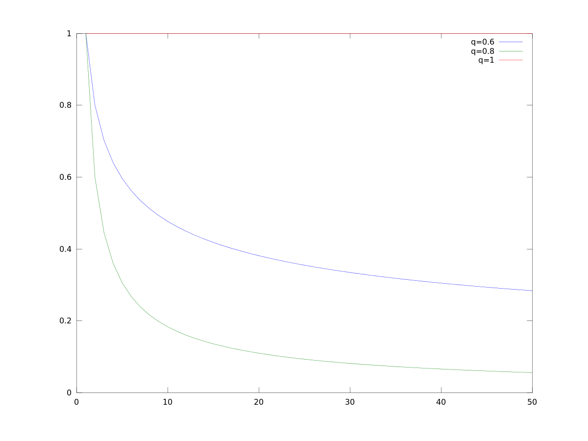
$y$ being the cost per unit, the total cost is now the sum of all our $y$, i.e.,

$$ \sum_{x=1}^n y(x) = \sum_{x=1}^n \max\left( a_1 x^{\log_2 q}, a_2 \right) $$

Clearly

$$ na_2 \le \sum_{x=1}^n y(x) \le na_1, \qquad (0\lt q\le1, \,\, 0\le a_2\le a_1) $$

For example, for $a_1=10$, $a_2=5$, and learning-rate varying from $q=1,\ldots,0.5$, $n=50$, we have the following bar-chart:

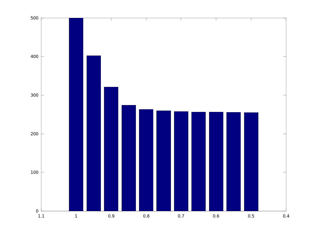
To make it specific, for a learning-rate of 90% you could calculate not with 500 man-days but rather 321 man-days, assuming you need 10 man-days initially, and at least 5 man-days, and have to produce 50 more or less similar artifacts.

Plotting with MATLAB/Octave. Getting numeric values with MATLAB or Octave uses code like this:

sum(  max(a1 * (1:n) .^ (log(q)/log(2)), a2)  )

Plotting individual costs per units in Octave goes like this

q1=log(0.8)/log(2)
q2=log(0.6)/log(2)
x=1:1:50
plot(x,x.^q1,"-;q=0.6;", x,x.^q2,"-;q=0.8;", x,x.^0,"-;q=1;")
print -color learn1.png -dpng

Plotting the sum goes like this

lq=[]; for q=0.5:0.05:1
     lq=horzcat(lq,sum( max(10*(1:50).^(log(q)/log(2)),5) ))
endfor
q=0.5:0.05:1
bar(q,lq)
set(gca, 'XDir', 'reverse')
print -color learn3.png -dpng

Conclusion. What can be seen from these figures is that you can beat your competition, i.e., offer your services for fewer man-days, if you incorporate learning curves.